(a)

On the axes of Fig. 2.3, sketch the variation with time of the power dissipated in a resistor by a sinusoidal alternating current during two cycles of the current.

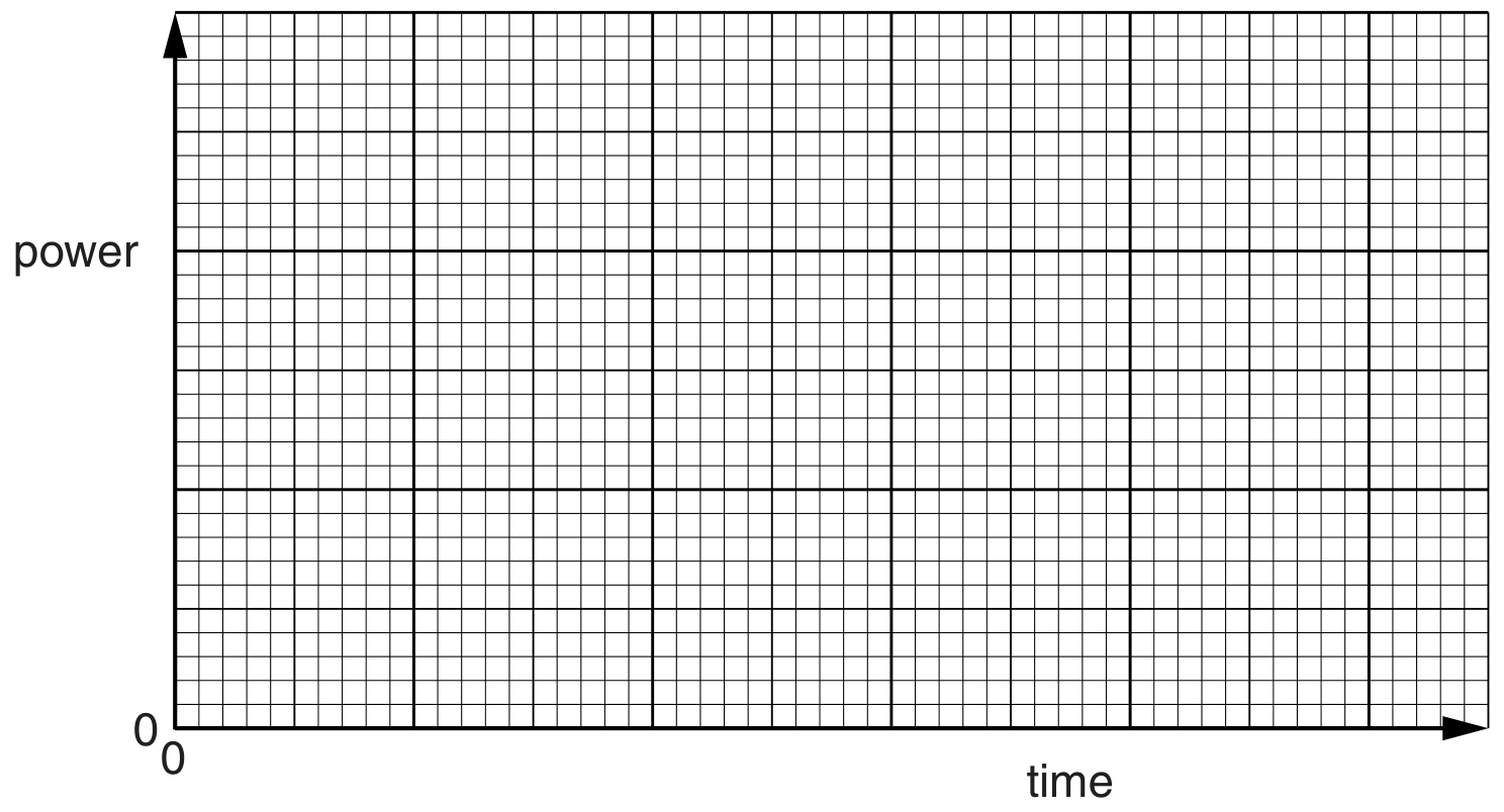
Fig. 2.3

[ 3 ]

(a)

A sinusoidal a.c. power supply has a maximum power of 16 W .

State the value of the mean power when the output of the power supply is:

[ 2 ]

(i)

full-wave rectified
mean power = W

[ 1 ]

(ii)

half-wave rectified.
mean power = W

[ 1 ]

[Maximum number: 3]

A Hall probe is placed a distance d from a long straight current-carrying wire, as illustrated in Fig.5.1.

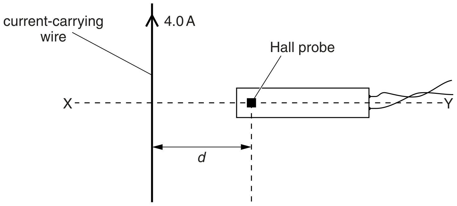
Fig. 5.1

The direct current in the wire is 4.0 A . Line XY is normal to the wire.
The Hall probe is rotated about the line X Y to the position where the reading $V_{H}$ of the Hall probe is maximum.

(a)

The Hall probe is now returned to its original position, a distance d from the wire. At this point, the magnetic flux density due to the current in the wire is proportional to the current.

For a direct current of 4.0 A in the wire, the reading of the Hall probe is 3.5 mV .
The direct current is now replaced by an alternating current of root-mean-square (r.m.s.) value 4.0 A . The period of this alternating current is T.

On the axes of Fig. 5.3, sketch the variation with time t of the reading of the Hall voltage $V_{\mathrm{H}}$ for two cycles of the alternating current. Give numerical values for $V_{\mathrm{H}}$ , where appropriate.

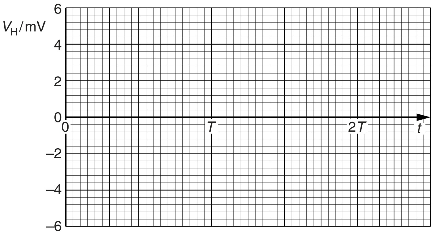
Fig. 5.3

[ 3 ]

[Maximum number: 4]

A sinusoidal alternating voltage supply is connected to a bridge rectifier consisting of four ideal diodes. The output of the rectifier is connected to a resistor R and a capacitor C as shown in Fig. 6.1.

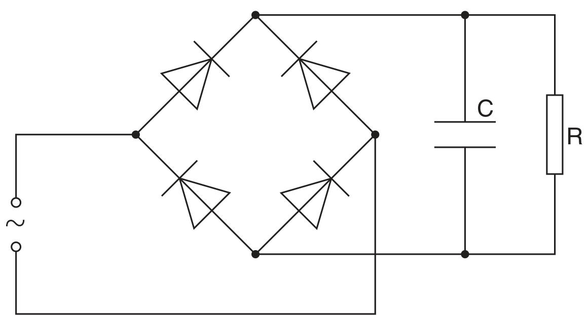
Fig. 6.1

The function of C is to provide some smoothing to the potential difference across R .
The variation with time t of the potential difference V across the resistor R is shown in Fig. 6.2.

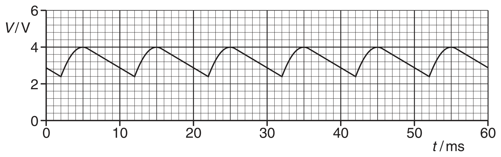
Fig. 6.2

(a)

Use Fig. 6.2 to determine, for the alternating supply,

[ 4 ]

(i)

the peak voltage,

peak voltage =V

[ 1 ]

(ii)

the root-mean-square (r.m.s.) voltage,
r.m.s. voltage = V

[ 1 ]

(iii)

the frequency. Show your working.

frequency =

[ 2 ]

[Maximum number: 4]

An electron in a metal rod moves randomly about a mean position. When an alternating voltage is applied to the ends of the rod, the mean position can be considered to oscillate with simple harmonic motion along the axis of the rod. Fig. 4.1 shows the variation with time t of the displacement x of the mean position from a fixed point on the axis of the rod.

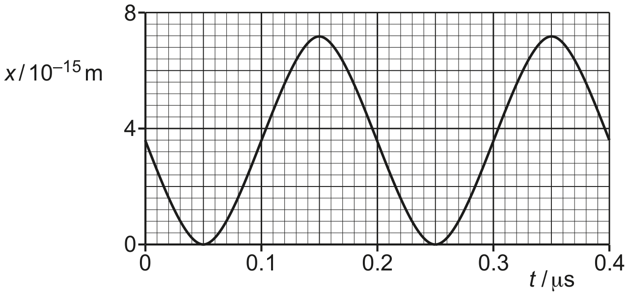
Fig. 4.1

(a)

The rod has a cross-sectional area of $4.3 \mathrm{~cm}^{2}$ and contains a number density of conduction electrons (charge carriers) of $8.5 \times 10^{28} \mathrm{~m}^{-3}$ .

All of the conduction electrons in the rod may be assumed to be oscillating in phase with, and with the same amplitude as, the oscillation shown in Fig. 4.1.

[ 4 ]

(i)

On Fig. 4.2, sketch the variation of the current I in the rod with time t between t=0 and $t=0.40 \mu \mathrm{~s}$ .

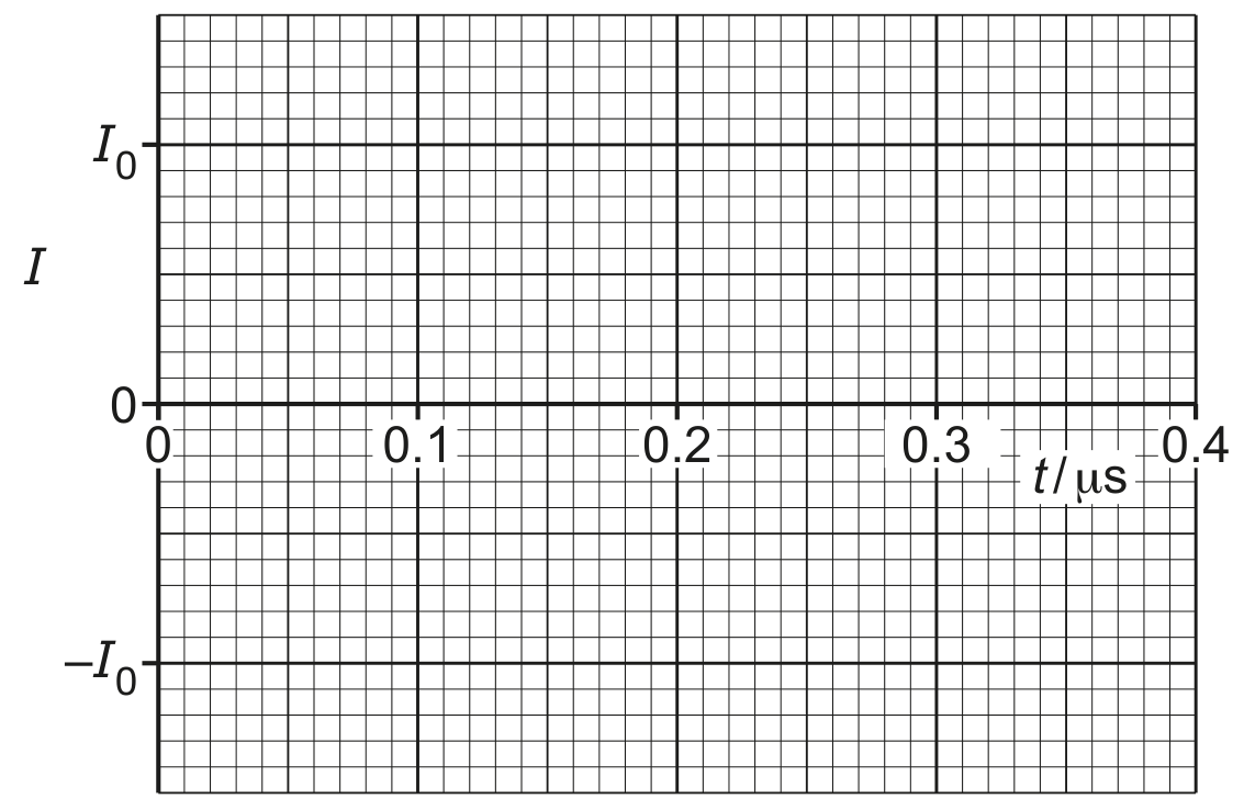
Fig. 4.2

[ 2 ]

(ii)

Use your answers in (a)(ii) and (b)(i) to determine an expression for I in terms of t, where I is in A and t is in s .

[ 1 ]

(iii)

Determine the root-mean-square (r.m.s.) current in the rod.
r.m.s. current = A

[ 1 ]

[Maximum number: 2]

A sinusoidal alternating potential difference (p.d.) from a supply is rectified using a single diode. The variation with time t of the rectified potential difference V is shown in Fig. 5.1.

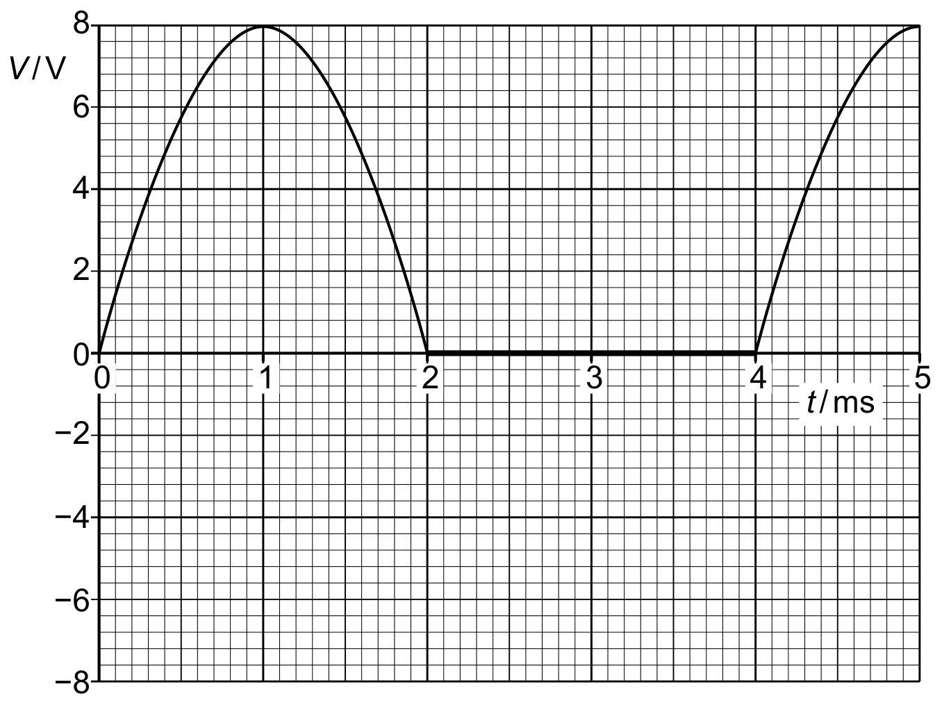
Fig. 5.1

(a)

(i)

Determine the root-mean-square (r.m.s.) value of the supply potential difference before rectification.
r.m.s. potential difference = \\ V

[ 2 ]

(a)

A low frequency alternating current is now passed through the wire in (b). The root-mean-square (r.m.s.) value of the current is 5.6 A .

Describe quantitatively the variation of the reading seen on the balance.

[ 2 ]

[Maximum number: 3]

A stiff straight copper wire XY is held fixed in a uniform magnetic field of flux density $2.6 \times 10^{-3} \mathrm{~T}$ , as shown in Fig. 6.1.

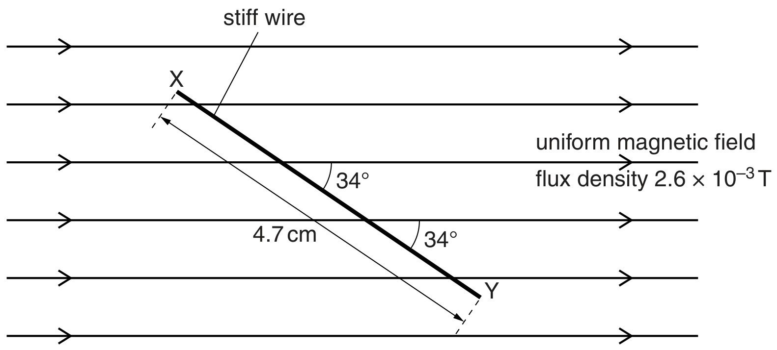
Fig. 6.1

The wire X Y has length 4.7 cm and makes an angle of $34^{\circ}$ with the magnetic field.

(a)

The current in the wire is now changed to an alternating current of r.m.s. value 1.7 A .

Determine the total variation in the force on the wire due to the alternating current.
variation in force = N

[ 3 ]

[Maximum number: 3]

Fig. 5.1 shows four diodes and a load resistor of resistance $1.2 \mathrm{k} \Omega$ , connected in a circuit that is used to produce rectification of an alternating voltage.

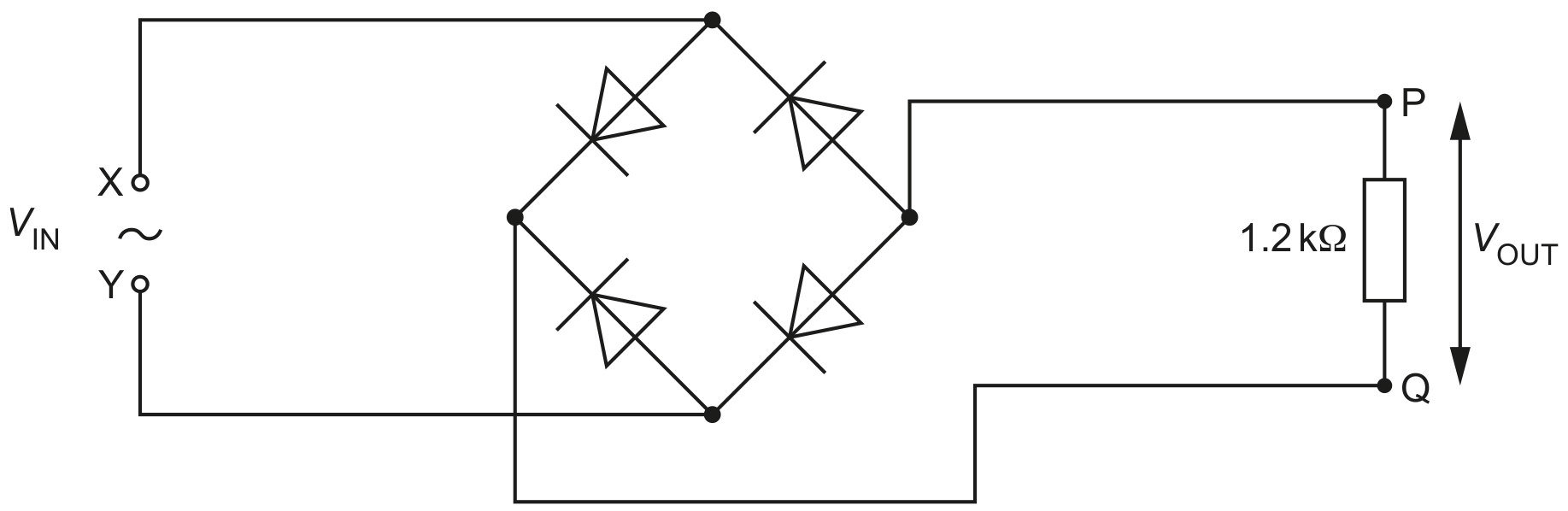
Fig. 5.1

(a)

A sinusoidal alternating voltage $V_{\text {IN }}$ is applied across the input terminals X and Y. The variation with time t of $V_{\text {IN }}$ is given by the equation

V_{\text {IN }}=6.0 \sin 25 \pi t

where $V_{\text {IN }}$ is in volts and t is in seconds.

[ 3 ]

(i)

The magnitude of the output voltage $V_{\text {OUT }}$ varies with t as shown in Fig. 5.2.

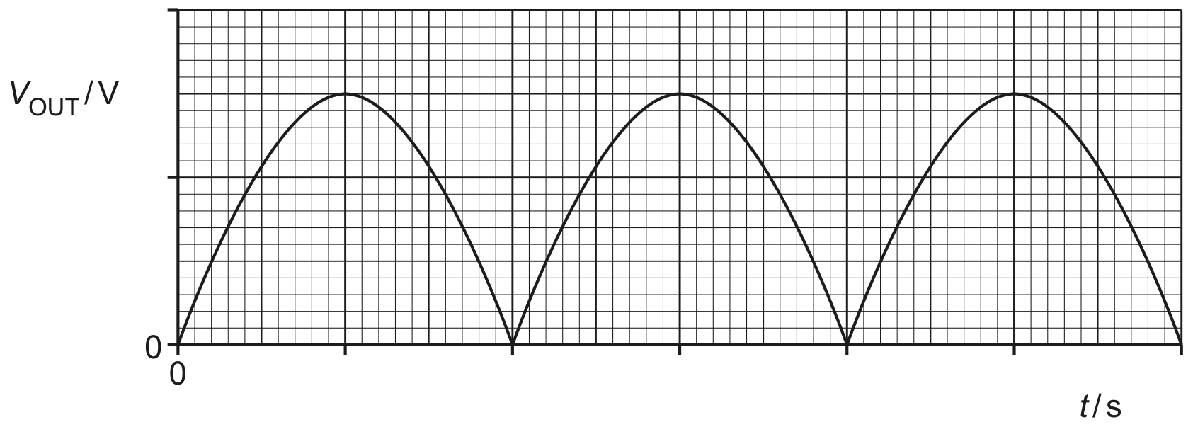
Fig. 5.2

On Fig. 5.2, label both of the axes with the correct scales. Use the space below for any working that you need.

[ 3 ]

[Maximum number: 4]

An alternating current supply is connected in series with a resistor R, as shown in Fig. 6.1.

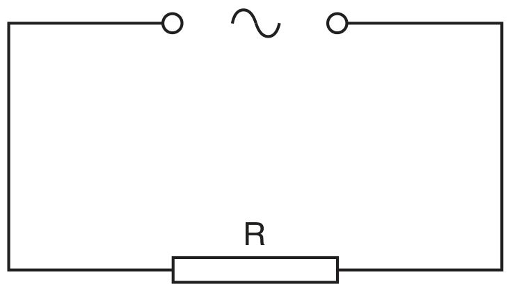
Fig. 6.1

The variation with time t (measured in seconds) of the current I (measured in amps) in the resistor is given by the expression

I=9.9 \sin (380 t)

(a)

For the current in the resistor R , determine

[ 4 ]

(i)

the frequency,
frequency = Hz

[ 2 ]

(ii)

the r.m.s. current.
r.m.s. current = A

[ 2 ]