D3.2.21 (HL)—Chi-squared test
The chi-squared test compares observed and expected genetic results to judge whether differences could be due to chance in inheritance problems.
- Syllabus
- First assessment 2025
- Objective
- D3.2.21
- Level
- HL
The chi-squared test compares observed and expected genetic results to judge whether differences could be due to chance in inheritance problems.

Coverage 2019–2021 · Updated 16 Jul 2026
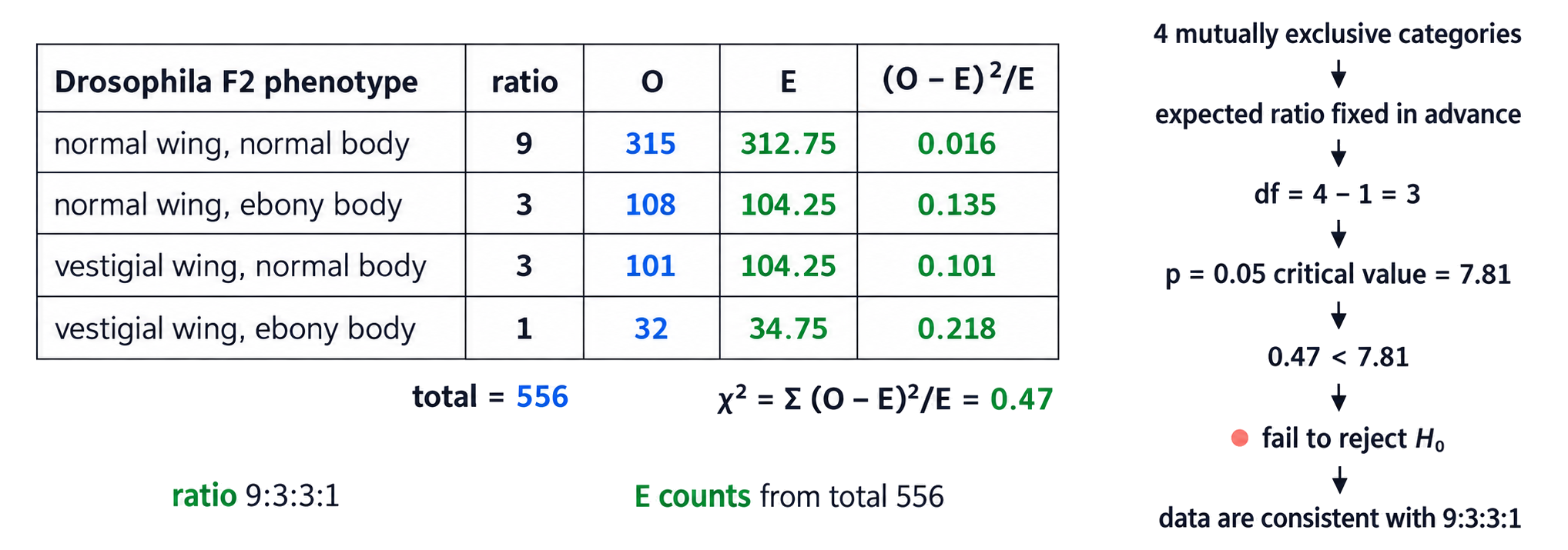
A chi-squared goodness-of-fit test asks whether differences between observed and expected dihybrid counts are larger than expected from chance sampling.
χ2=Σ((O−E)2/E),whereOiseachobservedcountandEisitsexpectedcount.χ2hasnounit;degreesoffreedom=numberofcategories−1.
State H₀: observed counts fit the stated Mendelian ratio; H₁: they do not. Convert the ratio to expected counts, calculate and sum each contribution, then compare χ² with the critical value at p = 0.05.
In local Question Bank record 10900, a four-category 1:1:1:1 model gives E = 575 in each category and df = 3. The supplied χ² = 1002.6 exceeds the p = 0.05 critical value 7.815, so reject H₀: the observed ratio differs significantly from expectation.
Failing to reject H₀ does not prove the model; rejecting it does not by itself identify linkage or another cause. Check assumptions, expected counts and experimental design.
This objective is assessed through structured response.
Build the answer around this relationship: Chi-squared compares observed counts with expected counts.
Representative question
The chi-squared value was calculated as shown. Deduce, with reasons, whether the observed ratio differed significantly from the expected Mendelian ratio.
| Probability | |||||||||||
|---|---|---|---|---|---|---|---|---|---|---|---|
| Degrees of freedom | 0.995 | 0.975 | 0.20 | 0.10 | 0.05 | 0.025 | 0.02 | 0.01 | 0.005 | 0.002 | 0.001 |
| 1 | 0.00004 | 0.001 | 1.642 | 2.706 | 3.841 | 5.024 | 5.412 | 6.635 | 7.879 | 9.550 | 10.828 |
| 2 | 0.010 | 0.051 | 3.219 | 4.605 | 5.991 | 7.378 | 7.824 | 9.210 | 10.597 | 12.429 | 13.816 |
| 3 | 0.072 | 0.216 | 4.642 | 6.251 | 7.815 | 9.348 | 9.837 | 11.345 | 12.838 | 14.796 | 16.266 |
| 4 | 0.207 | 0.484 | 5.989 | 7.779 | 9.488 | 11.143 | 11.668 | 13.277 | 14.860 | 16.924 | 18.467 |
| 5 | 0.412 | 0.831 | 7.289 | 9.236 | 11.070 | 12.833 | 13.388 | 15.086 | 16.750 | 18.907 | 20.515 |
| 6 | 0.676 | 1.237 | 8.558 | 10.645 | 12.592 | 14.449 | 15.033 | 16.812 | 18.548 | 20.791 | 22.458 |
| 7 | 0.989 | 1.690 | 9.803 | 12.017 | 14.067 | 16.013 | 16.622 | 18.475 | 20.278 | 22.601 | 24.322 |
a
yes/observed ratio did differ significantly «from the expected Mendelian ratio»
OR expected ratio is 1:1:1:1 / 575 of each type / 25 % of each type
b
3 degrees of freedom
c
critical value is 7.815 «at the 5\% level / 11.345 «at the 1\% level»
d
chi-squared value «of 1002.6» exceeds the critical value
HL D3.2 is secure when chromosome behaviour explains the ratios: segregation and independent assortment produce unlinked dihybrid expectations, gene loci explain linkage, recombinants reveal crossing over, and chi-squared decides whether observed counts fit the expected model.
HL inheritance transfer is about deciding whether the expected ratio should be Mendelian or linked, then testing the evidence. Start from meiosis and gene location, predict gametes or ratios, identify parental and recombinant classes, and use chi-squared when observed counts need a statistical conclusion.