D4.1.13 (HL)—Hardy-Weinberg equation

The Hardy-Weinberg equation predicts genotype frequencies from allele frequencies when a population is not evolving in evolving populations in evolving populations.

Syllabus
First assessment 2025
Objective
D4.1.13
Level
HL

Exam analysis

Chance of appearing7%of analysed past papers
Latest appearanceNovember 2025
Most common paperPaper3
Typical marks2–3

Common command terms

  • Outline
  • Discuss

Recent exam appearances

November 2025Paper1A ["HL"] · TZ338[ 1 ]D4.1.13 (HL)—Hardy-Weinberg equation
May 2025Paper2 ["HL"] · TZ29(b)[ 3 ]D4.1.13 (HL)—Hardy-Weinberg equation
May 2025Paper1B ["HL"] · TZ14(d)[ 3 ]D4.1.13 (HL)—Hardy-Weinberg equation
May 2015Paper3 ["HL"] · TZ23[ 6 ]D4.1.13 (HL)—Hardy-Weinberg equation
May 2014Paper3 ["HL"] · TZ12(b)(i)[ 2 ]D4.1.13 (HL)—Hardy-Weinberg equation

Coverage 2012–2025 · Updated 16 Jul 2026

Hardy–Weinberg Separates Allele Frequencies from Genotype Frequencies

HL only
Symbol Meaning for two alleles A and a
p frequency of A
q frequency of a
p² expected frequency of AA
2pq expected frequency of Aa
q² expected frequency of aa

p+q=1p+q=1

p2+2pq+q2=1p^2+2pq+q^2=1

p and q are allele frequencies; p², 2pq and q² are genotype frequencies. The equations do not require p to represent the dominant allele.

A Recessive Phenotype Reveals q², Not q

HL only
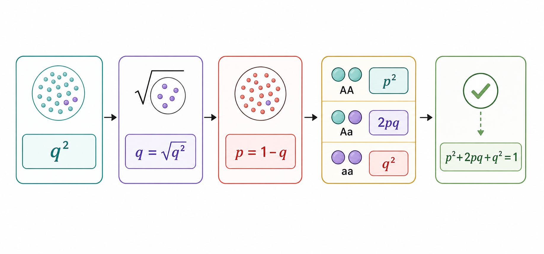
  1. Convert the recessive phenotype count to a frequency; under complete dominance this is q².
  2. Calculate q = √q².
  3. Calculate p = 1 − q.
  4. Calculate expected genotype frequencies p², 2pq and q².
  5. Check that the three genotype frequencies sum to 1.

This inference is valid only when the population and locus satisfy the Hardy–Weinberg model and the recessive phenotype identifies homozygous recessives accurately.

A Hardy–Weinberg workflow starts from observed q squared, takes a square root for q, calculates p, then predicts p squared, 2pq and q squared and checks their sum.

Worked Hardy–Weinberg Example: 35% Recessive Phenotype

HL only
Quantity Calculation Result
q² observed non-taster frequency 0.35
q √0.35 0.592
p 1 − 0.592 0.408
p² 0.408² 0.166
2pq 2 × 0.408 × 0.592 0.483
check 0.166 + 0.483 + 0.350 0.999 ≈ 1

In 200 people, expected counts are approximately 33 homozygous dominant, 97 heterozygous and 70 homozygous recessive after multiplying each frequency by 200.

Keep extra digits until the final answer. Early rounding makes the genotype frequencies fail to sum closely to 1.

Population Genetics Measures How Selection and Other Forces Change Gene Pools

HL only

count allele copies in the gene pool → establish p and q → use Hardy–Weinberg as a no-change expectation → compare observed genotype or allele frequencies across generations → use phenotype, fitness and population evidence to identify selection or another evolutionary force

Pattern or action First model to examine
mean shifts toward one extreme directional selection
variance narrows around intermediate values stabilizing selection
both extremes rise and intermediates fall disruptive selection
observed genotypes differ from p²:2pq:q² one or more equilibrium assumptions may be violated
humans repeatedly choose parents artificial selection

Keep description, calculation and cause separate. A changed distribution describes an outcome; allele counts quantify evolution; causal claims require evidence about inheritance, survival, mating, migration, drift or deliberate breeding.

Hardy-Weinberg equation

HL only

[ 3 ]

Discuss the use of the Hardy-Weinberg equation in population genetics studies.

Concept essentials

  • p and q are allele frequencies that add to one.
  • p squared, two pq and q squared are expected genotype frequencies.
  • Hardy-Weinberg calculations depend on equilibrium assumptions.