Continuity and Change links inheritance, regulation, reproduction, selection and environmental change to explain stability and transformation in cells, organisms and populations.
Syllabus
First assessment 2025
Section
—
Level
HL
Exam analysis
Published Concept evidence in Continuity and Change repeatedly connects genetic mechanisms, cell division, inheritance, regulation and selection. The strongest pattern is explaining how information is maintained, altered and acted on across cells, organisms and populations.
DNA replication copies genetic information through template strands, complementary pairing, enzyme action, proofreading, and laboratory amplification or separation techniques used to analyse DNA.
Syllabus
First assessment 2025
Topic
D1.1
Level
HL
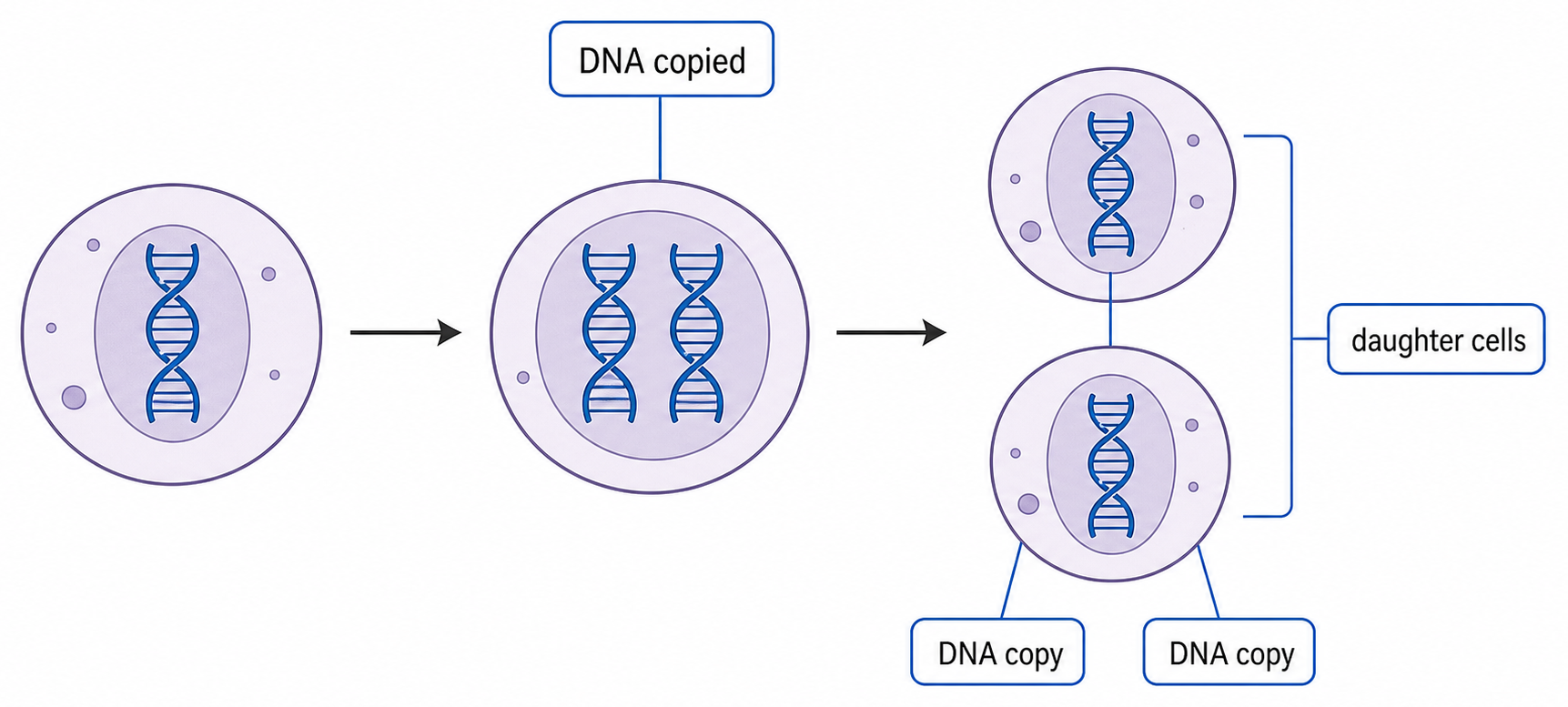
DNA Must Be Copied Before a Cell Divides
DNA replication produces a second DNA molecule with the same base sequence as the original, apart from rare errors.
chromosome DNA → replication during interphase → two DNA copies → cell division → one complete genome enters each daughter cell
Biological context
Why replication is required
reproduction
genetic information passes to new cells or offspring
growth
cell number increases without losing the genome
tissue replacement
new cells inherit the instructions needed for their function
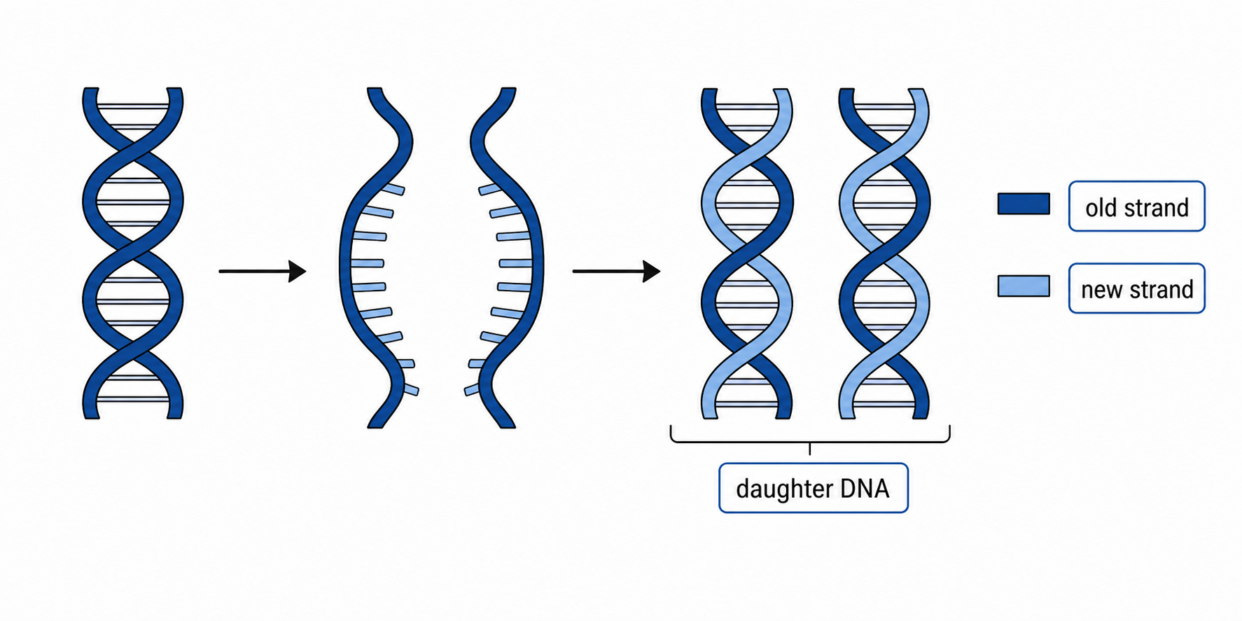
Each Old DNA Strand Templates a New Complement
Exposed template base
New nucleotide added
A
T
T
A
C
G
G
C
The sequence of each original strand determines a complementary new sequence. The two products therefore preserve the original base-pair sequence.
Semi-conservative means that each daughter double helix contains one parental strand and one newly synthesized strand—not that half of every strand is old.
Meselson and Stahl Tested the Strand-Distribution Models
E. coli were first grown with ¹⁵N so their DNA was heavy, then transferred to ¹⁴N medium. DNA from successive generations was separated by density-gradient centrifugation.
Sample
Observed DNA bands
What the result shows
before transfer
one heavy band
all DNA initially contains ¹⁵N
after one replication
one intermediate band
every molecule contains heavy and light material
after two replications
one intermediate + one light band
hybrid molecules persist while fully light molecules appear
The one-generation intermediate band rejects conservative replication, which predicts separate heavy and light bands. The two-generation pattern matches semi-conservative copying.
The isotopes label nitrogen in DNA; they do not make replication radioactive. Both ¹⁵N and ¹⁴N are stable isotopes.
Helicase Exposes Templates; DNA Polymerase Builds Backbones
1
Helicase unwinds the double helix and breaks the hydrogen bonds between complementary bases, exposing two template strands.
2
Free DNA nucleotides align with exposed bases by complementary base pairing.
3
DNA polymerase joins adjacent nucleotides by forming phosphodiester bonds in the sugar–phosphate backbone of each new strand.
Enzyme
Bonds affected
Job
helicase
hydrogen bonds between bases
separates the two strands
DNA polymerase
phosphodiester bonds within a new strand
links nucleotides into a backbone
Helicase does not elongate DNA. It opens the template; DNA polymerase performs strand synthesis.
Reconstruct the Core Replication Argument
need two genomes → helicase separates the original strands → each old strand acts as a template → complementary nucleotides pair → DNA polymerase links the new backbone → two matching double helices form
Feature to check
Correct outcome
sequence
complementary copying preserves the base-pair sequence
strand origin
each product has one old strand and one new strand
biological result
a complete genome can pass to each daughter cell
A model explains how copying could occur; the Meselson–Stahl band pattern provides experimental evidence that the one-old-one-new strand distribution actually occurs.
PCR Selects a DNA Region with Two Primers
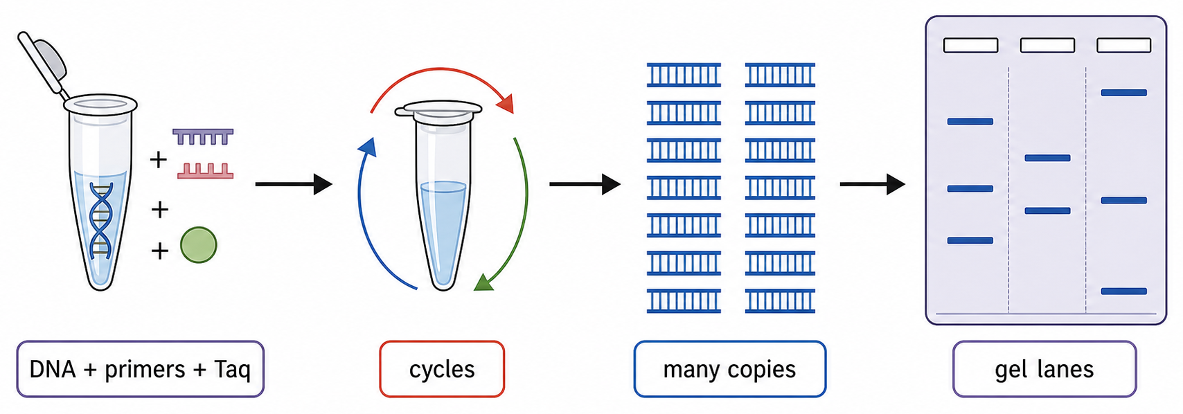
The polymerase chain reaction (PCR) amplifies a selected DNA region in vitro, producing enough copies for detection or analysis.
Component
Job
template DNA
contains the target sequence
two DNA primers
bind on opposite strands at the target's ends and provide free 3′ ends
free DNA nucleotides
become the new strands
Taq polymerase
extends primers and remains active after high-temperature heating
Primer sequences determine which interval is copied. The target's flanking sequences must therefore be known well enough to design complementary primers.
One PCR Cycle Separates, Primes and Extends DNA
1
Denaturation, about 95 °C: hydrogen bonds break and double-stranded DNA separates into templates.
2
Annealing, a lower temperature: primers bind to complementary sequences flanking the target.
3
Extension, about 72 °C: Taq polymerase adds nucleotides to each primer's 3′ end, synthesizing new DNA 5′→3′.
Heating begins the next cycle by separating the newly formed double strands. A thermal cycler repeats the temperature sequence automatically.
Cooling does not make DNA polymerase copy the target by itself. Cooling permits primer binding; polymerase extends only after a primer supplies a paired 3′ end.
Repeated PCR Cycles Amplify—But Not Perfectly
Nn=N0(2n)
In the ideal early cycles, each target molecule produces two copies per cycle. Starting from one target, 30 perfect doublings would give about one billion copies.
Taq polymerase comes from the thermophilic bacterium Thermus aquaticus. Its heat stability prevents the enzyme from being destroyed during repeated denaturation.
Limitation
Consequence
primers bind a similar non-target sequence
the wrong interval can be amplified
contamination supplies foreign DNA
contaminant DNA can also be copied
reagents become limiting and products reanneal
later cycles fall below ideal doubling
Taq lacks proofreading
some newly copied molecules contain errors
An Electric Field Separates DNA Fragments through a Gel
DNA samples are loaded into wells near the negative electrode of a porous agarose gel immersed in conducting buffer.
Phosphate groups give DNA a net negative charge, so fragments migrate through the gel toward the positive electrode when voltage is applied.
Fragment
Movement through gel pores
Final tendency after the same time
shorter
less hindered; moves faster
farther from the wells
longer
more hindered; moves slower
nearer the wells
DNA is colourless. A stain or labelled probe is needed to reveal separated fragments as bands.
For DNA fragments, charge gives a common migration direction; fragment length is the main variable responsible for separation through the gel.
Band Position Reports Fragment Length; Alignment Reports a Match
Observation
Interpretation
band farther from wells
shorter DNA fragments
bands at the same height in two lanes
fragments of the same measured length
more intense band
more stained DNA at that position, not a longer fragment
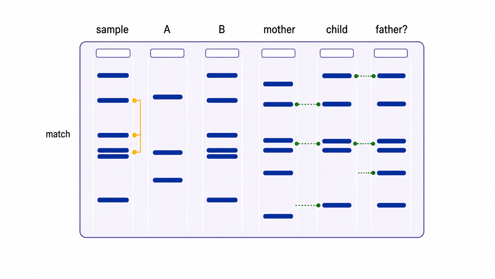
Compare lanes horizontally, one band position at a time. A profile comparison uses a pattern across many variable markers, not one matching band.
A same-height band supports a shared fragment length; it does not by itself prove that every base in the fragments is identical.
DNA Profiles Compare Several Variable Markers
collect and preserve samples → extract DNA → amplify selected STR or VNTR markers by PCR → separate products by electrophoresis → compare band or peak patterns
Result
Supported conclusion
Not established by the profile alone
questioned sample differs at a reliable marker
that reference individual is excluded
who left the sample
all tested markers match
the samples may share a source
when or how the DNA arrived
Match strength increases when more independent, variable markers agree and when the matching pattern is rare in the relevant population.
Contamination, mixed samples, degraded DNA and laboratory error can weaken the inference. Controls and careful sample handling are part of the evidence.
A Child's Markers Must Be Accounted for by Both Parents
At each tested marker, a child inherits one allele from the biological mother and one from the biological father.
Start with the child's pattern → account for bands or alleles shared with the known parent → compare every remaining child marker with the possible other parent.
Comparison
Inference
a required child marker is absent from the possible parent
exclude that person at that marker, after checking data quality
all non-maternal child markers are present in the possible father
parentage is supported, with strength depending on marker number and frequencies
Close relatives share more DNA than unrelated people. Parentage conclusions use multiple markers and probability, not a visual impression from one or two bands.
Follow DNA from a Tiny Sample to a Qualified Conclusion
Stage
Question answered
Key control
primer design
which region will be copied?
complementary, target-specific flanking sequences
PCR
is there enough target DNA to analyse?
positive and negative controls; contamination prevention
electrophoresis
what fragment lengths are present?
ladder and correct electrode orientation
profile comparison
are patterns consistent with a shared source or inheritance?
enough informative markers and relevant frequencies
PCR changes quantity; electrophoresis changes position; interpretation changes neither. Each step supports a different claim.
A laboratory match is evidence of consistency. The final conclusion must remain limited by sample quality, contamination risk, marker informativeness and the biological question being tested.
DNA Polymerase Extends a Strand Only at Its 3′ End
HL only
The two DNA strands are antiparallel: one runs 5′→3′ while its complement runs 3′→5′.
DNA polymerase forms a phosphodiester bond between the growing strand's free 3′-OH and the incoming nucleotide. New DNA therefore grows only 5′→3′.
Polymerase action
Direction
reads template
3′→5′
synthesizes new strand
5′→3′
Antiparallel Templates Force Two Replication Patterns
HL only
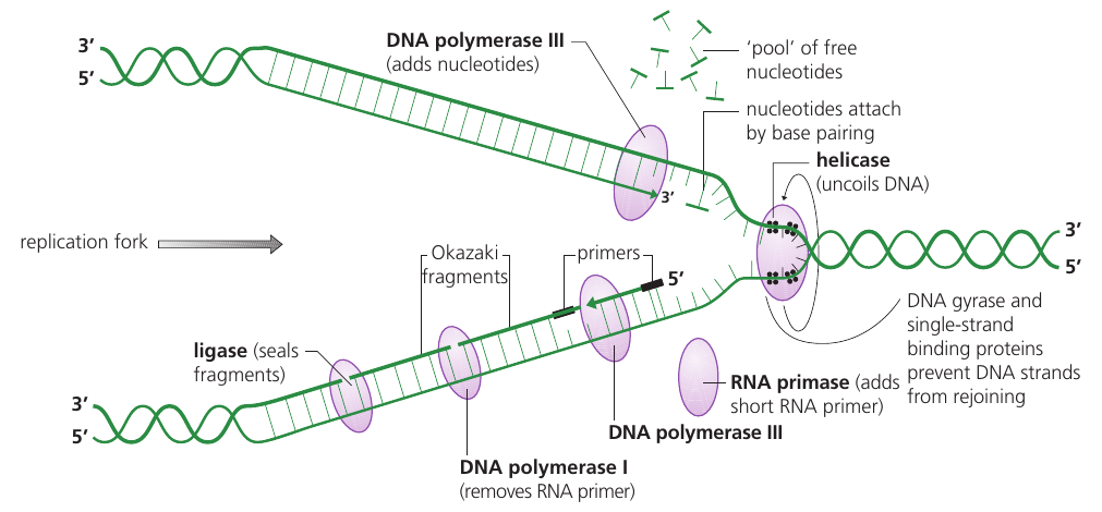
Both templates are exposed at the same fork, but DNA polymerase can extend each new strand only 5′→3′.
On one template, 5′→3′ synthesis follows the advancing fork, so polymerase can remain behind helicase and synthesize continuously.
On the opposite template, 5′→3′ synthesis points away from the fork. Newly exposed template must be copied in short sections that begin repeatedly near the fork.
The lagging strand is discontinuous because of antiparallel geometry and polymerase directionality—not because its polymerase is slower.
Leading Is Continuous; Lagging Uses Okazaki Fragments
HL only
Feature
Leading strand
Lagging strand
relation to fork movement
synthesis proceeds toward the fork
each fragment is synthesized away from the fork
synthesis pattern
continuous
discontinuous
RNA primers at one fork
one initial primer
repeated primers
DNA product before processing
one continuous new strand
multiple Okazaki fragments
ligase requirement
not required to join Okazaki fragments
joins processed fragments
Both new strands are synthesized simultaneously and both grow 5′→3′. The difference is continuous versus fragment-by-fragment synthesis.
The leading strand also needs an RNA primer to begin. Repeated priming is distinctive of the lagging strand.
Primase Starts; DNA Polymerase III Extends
HL only
1
DNA polymerase III cannot start a strand from unlinked nucleotides; it needs an existing paired chain with a free 3′-OH.
Primase is an RNA polymerase that synthesizes a short RNA primer complementary to the DNA template. It can start without a pre-existing 3′ end.
2
DNA polymerase III binds at the primer's 3′ end and adds complementary DNA nucleotides, extending the new strand 5′→3′.
New strand
Primase action
DNA polymerase III action
leading
makes one initial primer
extends continuously
lagging
makes a new primer for each fragment
extends each Okazaki fragment
DNA Polymerase I Replaces Primers; Ligase Seals Nicks
HL only
1
DNA polymerase I removes each RNA primer and replaces its RNA nucleotides with DNA nucleotides.
After replacement, adjacent DNA sections contain the correct nucleotides but remain separated by a nick: one missing phosphodiester bond in the sugar–phosphate backbone.
2
DNA ligase catalyses formation of the missing phosphodiester bond, joining adjacent DNA fragments into one continuous strand.
Enzyme
Changes nucleotide identity?
Joins a final backbone gap?
DNA polymerase I
yes—RNA is replaced with DNA
leaves a nick between sections
DNA ligase
no
yes—seals the nick
Replication Enzymes Hand the Growing DNA from One Job to the Next
HL only
1
Helicase: separates the parental strands at the replication fork.
2
Primase: makes an RNA primer that supplies a free 3′-OH.
3
DNA polymerase III: extends complementary DNA from the primer.
4
DNA polymerase I: removes the RNA primer and replaces it with DNA.
5
DNA ligase: seals the remaining nick between DNA sections.
Material present
Next enzyme needed
paired template but no starting chain
primase
RNA primer with free 3′ end
DNA polymerase III
RNA segment embedded before DNA
DNA polymerase I
adjacent DNA sections with a nick
DNA ligase
DNA Polymerase III Proofreads the Growing 3′ End
HL only
1
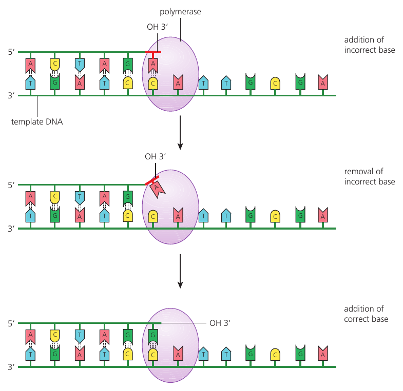
A newly added nucleotide that does not pair correctly distorts the polymerase–DNA structure and stalls extension.
2
DNA polymerase III shifts the 3′ end to its proofreading site, where exonuclease activity removes the mismatched nucleotide.
3
The corrected 3′ end returns to the polymerizing site; the complementary nucleotide is added and 5′→3′ synthesis resumes.
Proofreading greatly reduces replication errors and therefore mutation rate, but it cannot make replication completely error-free.
Solve a Replication Fork from Direction to Fidelity
HL only
Clue at the fork
Consequence
polymerase can add only to a 3′ end
every new segment grows 5′→3′
synthesis can follow helicase
leading strand is continuous
synthesis must restart as template is exposed
lagging strand uses repeated primers and Okazaki fragments
an RNA primer remains
DNA polymerase I replaces it with DNA
two DNA sections meet at a nick
ligase seals the phosphodiester bond
the terminal base is mismatched
DNA polymerase III removes and replaces it
helicase opens → primase starts → DNA polymerase III extends → DNA polymerase I replaces RNA → ligase seals → polymerase III proofreading corrects many terminal mismatches
Directionality creates the leading–lagging difference. Enzyme handoffs solve that geometry, while complementary pairing plus proofreading preserves sequence fidelity.
DNA replication
[ 8 ]
Growth in living organisms includes replication of DNA. Explain DNA replication.
Semi-conservative replication
[ 3 ]
Outline the reason that DNA replication is described as semi-conservative.
Role of helicase and DNA polymerase
[ 1 ]
What is a function of the enzyme helicase?
PCR and gel electrophoresis
[ 4 ]
Describe the polymerase chain reaction (PCR).
Applications exam focus
[ 4 ]
Outline the process of DNA profiling.
DNA polymerase directionality
HL only
[ 1 ]
How does DNA replicate?
Leading vs. lagging strand
HL only
[ 1 ]
What is a difference between the leading and lagging strands in DNA replication?
Functions in replication
HL only
[ 3 ]
Describe the function of three named enzymes involved in DNA replication.
DNA proofreading
HL only
[ 4 ]
Explain how mutation is avoided during DNA replication.
D1.2 Protein synthesis
Protein synthesis links DNA information to functional proteins through transcription, RNA processing, translation, genetic-code reading and post-translational modification in cells.
Syllabus
First assessment 2025
Topic
D1.2
Level
HL
mRNA Carries a Working Copy of Selected DNA Information
Chromosomal DNA is the long-term information store. Protein synthesis instead uses a short-lived messenger RNA (mRNA) copy of a selected gene.
selected gene in DNA → complementary mRNA copy → mRNA reaches a ribosome → nucleotide sequence directs amino-acid order
A working copy solves two problems:
The original DNA sequence remains protected and reusable.
Many mRNA copies can be made, so one gene can support repeated protein production.
mRNA carries information; it is not converted into protein matter. The ribosome reads its sequence while amino acids are joined into a separate molecule.
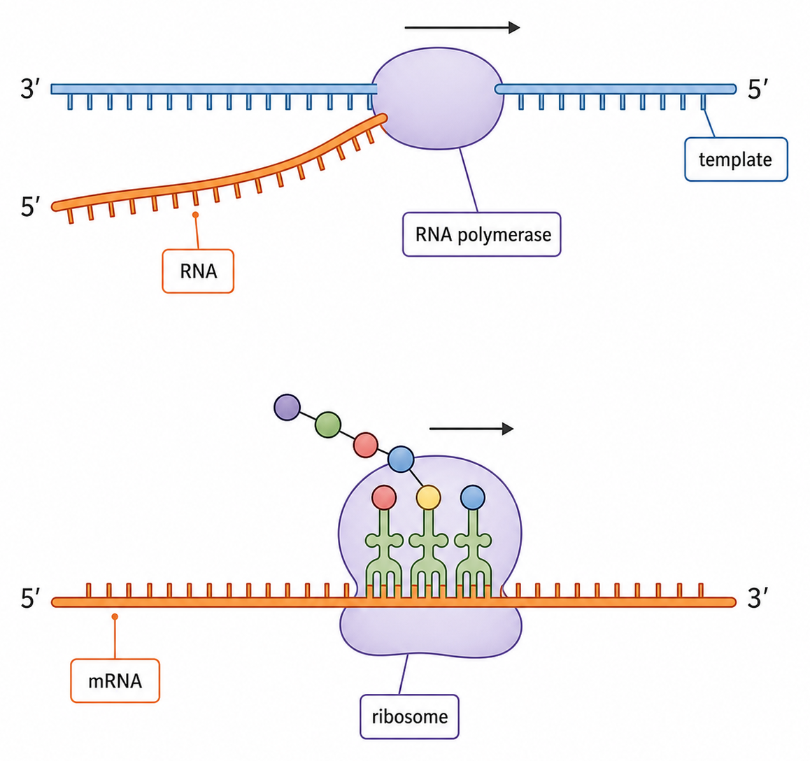
RNA Polymerase Builds mRNA from One DNA Template Strand
1
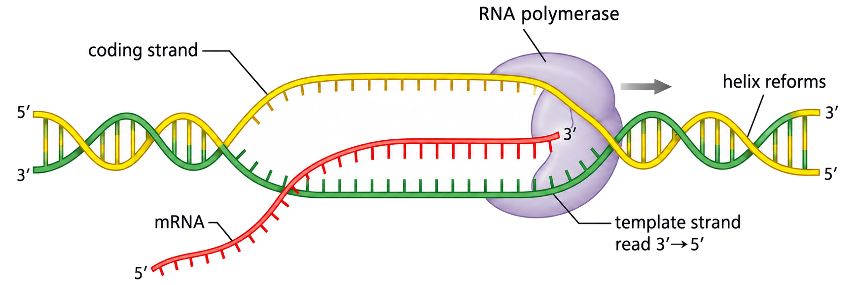
RNA polymerase binds near the gene and opens a short region of the DNA double helix, exposing the template strand.
2
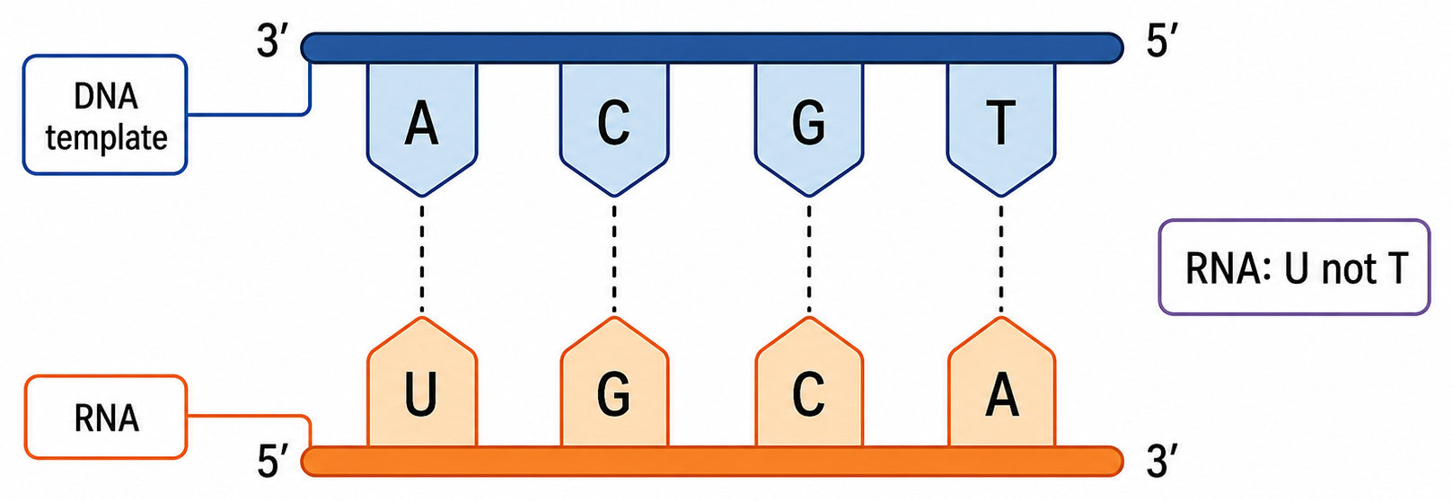
Free RNA nucleotides align by complementary base pairing: DNA A pairs with RNA U, DNA T with RNA A, and C with G.
3
RNA polymerase joins the RNA nucleotides into a sugar–phosphate backbone. The mRNA separates, and the DNA strands pair again.
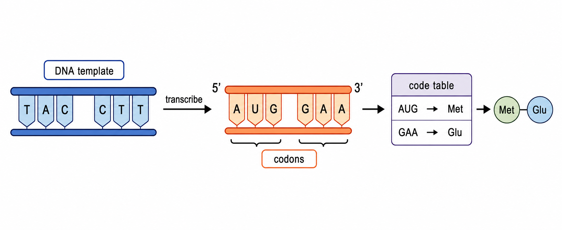
Template DNA Determines the mRNA Sequence
Strand
Relationship to the new mRNA
DNA template
antiparallel and complementary
DNA coding strand
same base order as mRNA, except DNA has T where RNA has U
DNA template: 3′–TAC CTT GCG–5′
mRNA: 5′–AUG GAA CGC–3′
Codon tables are read from mRNA 5′→3′. Do not look up a DNA template triplet directly.
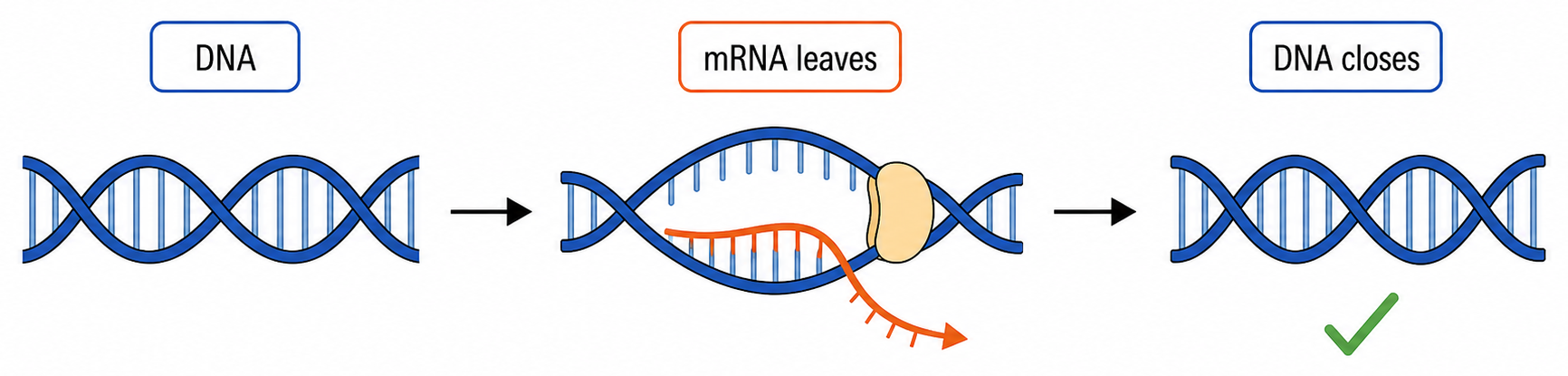
Transcription Opens DNA Locally and Leaves Its Sequence Unchanged
Hydrogen bonds between complementary bases can break and re-form. This lets a short DNA region open temporarily without breaking the covalent sugar–phosphate backbones.
After the mRNA leaves, the original complementary DNA strands pair again. The gene's base sequence is conserved and can be transcribed repeatedly.
Transcription copies one gene region into RNA; it does not duplicate the whole DNA molecule and does not consume the template strand.
Selective Transcription Controls Which Proteins a Cell Can Make
Gene expression is the use of gene information to produce a functional RNA or polypeptide. Transcription is a major control point because an untranslated gene cannot supply mRNA to ribosomes.
Transcription state
Immediate consequence
Possible protein outcome
gene active
mRNA is produced
translation can occur
gene inactive
little or no mRNA is produced
little or no corresponding polypeptide is made
Most cells in one organism contain the same genome, but different cell types transcribe different gene sets. Their different protein mixtures produce different structures and functions.
Turning transcription on permits expression; it does not guarantee a fixed protein amount. RNA processing, translation and protein breakdown can also be regulated.
Reconstruct the Route from a Selected Gene to mRNA
gene selected → DNA opens locally → RNA polymerase reads one template strand → complementary RNA nucleotides are joined → mRNA leaves → DNA re-forms unchanged
Question
Correct check
Which DNA strand determines mRNA?
the template strand
Which base replaces thymine in RNA?
uracil
Which direction is mRNA written?
5′→3′
Why can the gene be reused?
DNA sequence and covalent backbones remain intact
The mRNA now carries codons in an order that a ribosome can translate into an amino-acid sequence.
Translation Converts Codon Order into Amino-Acid Order
Translation is the synthesis of a polypeptide whose amino-acid sequence is determined by the codon sequence of an mRNA.
mRNA codons read 5′→3′ → matching tRNAs deliver amino acids → ribosome forms peptide bonds → polypeptide grows from its amino end toward its carboxyl end
The immediate product is a polypeptide: a specific linear amino-acid sequence. Folding and later processing are needed before many polypeptides become functional proteins.
The genetic code determines amino-acid order, not the final three-dimensional shape directly. Shape emerges from interactions within the amino-acid sequence and its environment.
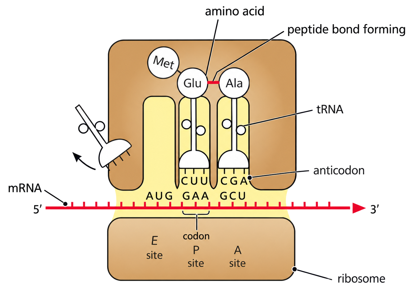
mRNA, tRNA and the Ribosome Divide Translation Work
Component
Information or material carried
Translation job
mRNA
ordered codons
supplies the sequence to be read
tRNA
one anticodon and its attached amino acid
matches a codon and delivers the corresponding amino acid
small ribosomal subunit
mRNA-binding site
positions the message for decoding
large ribosomal subunit
A, P and E sites
positions tRNAs and catalyses peptide-bond formation
Translation is accurate only when all three information links agree: the mRNA codon, the tRNA anticodon and the amino acid attached to that tRNA.
The ribosome does not choose amino acids by recognizing their chemical identity. It accepts charged tRNAs whose anticodons pair with the exposed codons.
Two Recognition Events Protect Amino-Acid Identity
At the ribosome, a tRNA anticodon pairs antiparallel with a complementary mRNA codon. This selects which tRNA can occupy the decoding site.
Before translation, a specific aminoacyl-tRNA synthetase attaches the correct amino acid to its matching tRNA. This charging step links anticodon identity to amino-acid identity.
Recognition
Example
What it secures
codon–anticodon pairing
mRNA 5′–AUG–3′ pairs with tRNA 3′–UAC–5′
the correct tRNA is selected
enzyme–tRNA/amino-acid recognition
methionine is attached to the initiator tRNA
the selected tRNA carries the correct amino acid
Complementary base pairing alone cannot check which amino acid is attached. Translation fidelity depends on both correct pairing and correct tRNA charging.
The Genetic Code Is Triplet, Degenerate and Nearly Universal
The genetic code has several linked properties:
Triplet: three mRNA bases form one codon.
Degenerate: most amino acids are specified by more than one codon.
Unambiguous: each codon specifies only one amino acid or stop signal.
Nearly universal: the same codons usually have the same meanings across organisms, with limited exceptions.
Punctuated: a start codon establishes the reading frame; stop codons end translation.
Degeneracy means some base substitutions are silent, but it does not mean one codon can represent several different amino acids.
Codon type
Function
AUG
usually codes for methionine and can establish the start of translation
UAA, UAG, UGA
stop signals recognized by release factors; they do not add an amino acid
Read the mRNA 5′→3′ before Using a Codon Table
1
If a DNA template is supplied, write the antiparallel complementary mRNA, replacing DNA A with RNA U.
2
Write the mRNA 5′→3′, locate the stated or biologically relevant start, and divide the sequence into consecutive triplets from that frame.
3
Look up each mRNA codon, record amino acids in order and stop when a stop codon is reached.
4
Template 3′–TAC CTT GCG ACT–5′ gives mRNA 5′–AUG GAA CGC UGA–3′, which translates as Met–Glu–Arg–Stop.
Elongation Repeats Until a Stop Codon Ends Translation
1
A charged tRNA with a complementary anticodon enters the A site beside the tRNA carrying the growing chain in the P site.
2
The ribosome catalyses a peptide bond, transferring the growing polypeptide to the amino acid on the A-site tRNA.
3
The ribosome moves one codon along the mRNA. The peptidyl-tRNA shifts to P, the empty tRNA shifts to E and exits, and the A site becomes available again.
4
The entry–bond–movement cycle repeats for successive codons. When a stop codon reaches the A site, no tRNA enters; a release factor releases the completed polypeptide and the ribosome dissociates.
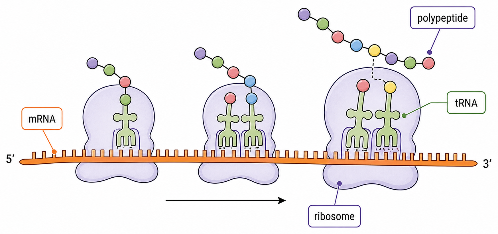
A Polysome Makes Several Copies from One mRNA at Once
A polysome is one mRNA being translated simultaneously by several ribosomes. Each ribosome starts near the 5′ end and moves toward the 3′ end.
All ribosomes read the same codon sequence, so they produce polypeptides with the same amino-acid order. Simultaneous translation increases the rate of protein production from that mRNA.
The ribosomes do not cooperate to make one long polypeptide. Each ribosome makes a separate copy.
A DNA Mutation Does Not Always Change the Protein
A mutation can alter a DNA base sequence. If the changed region is transcribed, it can alter an mRNA codon and therefore the amino-acid sequence or the timing of translation.
Codon outcome
Possible protein consequence
codon still specifies the same amino acid
no change to primary structure
codon specifies a different amino acid
altered side-chain interactions, folding or function
codon becomes a stop signal
shortened polypeptide
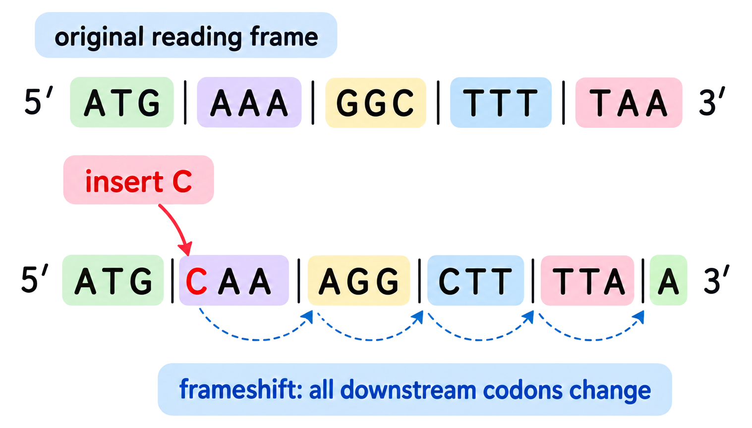
insertion or deletion shifts the reading frame
many downstream codons may change
Effect size depends on where the mutation occurs and what the affected amino acid does. A substitution at an active site or interaction surface can matter more than one in a tolerant region.
Mutation creates a possibility of changed protein structure; it does not guarantee harm. Some mutations are silent, neutral or beneficial in a particular environment.
One β-Globin Substitution Can Reshape a Red Blood Cell
1
In the sickle-cell allele, a β-globin DNA substitution changes an mRNA codon from GAG to GUG, replacing glutamate with valine in the polypeptide.
2
Glutamate is charged and hydrophilic; valine is non-polar. The replacement creates a hydrophobic patch on deoxygenated haemoglobin S.
3
Under low oxygen conditions, haemoglobin S molecules associate into long fibres. The fibres distort the red blood cell into a rigid sickle shape.
4
Rigid cells can block small blood vessels and are removed rapidly from circulation, reducing oxygen delivery and causing anaemia and painful crises.
The mutation does not directly bend the whole cell. It first changes one amino acid, which changes intermolecular interactions, which then changes cell shape under particular oxygen conditions.
Trace Information—and the Places Where It Can Change
Is the mRNA complementary to the template and written 5′→3′?
code table
Are mRNA codons grouped from the correct start?
tRNA selection
Does the anticodon pair and is the tRNA correctly charged?
elongation
Has the ribosome advanced one codon while the chain remains on the peptidyl-tRNA?
mutation
Did the codon, amino acid or reading frame actually change?
A sequence change matters biologically only through a causal path: altered primary structure → altered interactions or folding → altered protein activity → possible cellular or organism effect.
Information Is Read in Opposite Strand Directions but Built 5′→3′
HL only
Process
Molecule being read
Reading direction
Product growth or movement
transcription
DNA template
3′→5′
RNA is synthesized 5′→3′
translation
mRNA
5′→3′
ribosome moves toward the mRNA 3′ end; polypeptide grows N-terminus→C-terminus
Nucleotides are added to a free 3′ hydroxyl group, so every new nucleic-acid strand grows 5′→3′. The template must therefore be read antiparallel to the new strand.
A diagram arrow showing polymerase movement and an arrow showing new-strand growth refer to opposite strands; identify which molecule each arrow belongs to.
Promoters and Transcription Factors Assemble the Start Complex
HL only
A promoter is a DNA region that positions the transcription machinery near a gene's transcription start site. General transcription factors bind first and help recruit RNA polymerase.
Regulatory input
Binding relationship
Typical effect on initiation
activator transcription factor
binds a regulatory DNA sequence such as an enhancer
stabilizes or recruits the initiation machinery
repressor transcription factor
binds a regulatory sequence or interferes with the complex
reduces assembly or activity of the initiation machinery
Regulatory DNA may be far from the promoter in the linear sequence. DNA looping can bring bound factors into contact with promoter-associated proteins.
The combined transcription-factor state changes how often RNA polymerase initiates, altering the amount of pre-mRNA produced from the gene.
Non-Coding DNA Includes Several Functional Categories
HL only
Non-coding DNA is DNA that is not translated into a polypeptide sequence. Non-coding does not mean untranscribed, unused or without function.
Important non-coding categories include:
Regulatory sequences such as promoters and enhancers that affect transcription.
Introns that are transcribed into pre-mRNA and removed during splicing.
Genes for functional RNAs, including rRNA and tRNA, whose products are not translated.
Structural regions such as telomeres and centromeric DNA.
Repeated sequences, some functional and some with no known function.
An exon can include untranslated regions, so exon is not a synonym for protein-coding sequence. Likewise, an intron can influence regulation or splicing even though it is removed from mature mRNA.
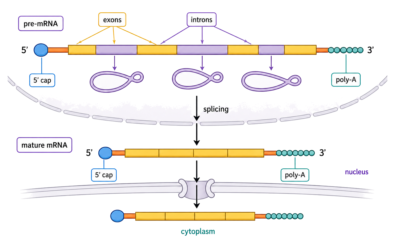
Capping, Polyadenylation and Splicing Produce Mature mRNA
HL only
Processing change
What happens
Main consequence
5′ cap
a modified nucleotide is added to the 5′ end
protects RNA and supports export and translation initiation
poly-A tail
many adenine nucleotides are added to the 3′ end
increases stability and supports export and translation
splicing
introns are removed and exons joined
creates a continuous mature RNA sequence for translation
pre-mRNA in nucleus → processing completed → mature mRNA exported through a nuclear pore → translation in cytoplasm
The poly-A tail is added after transcription; it is not copied from a long template-DNA sequence of thymine bases.
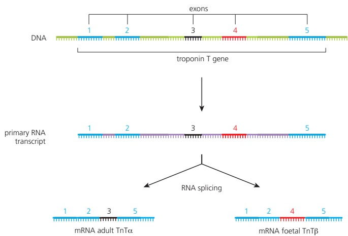
Alternative Splicing Changes Which Exons Reach the Ribosome
HL only
In alternative splicing, the same pre-mRNA is spliced in different patterns, so different exon combinations are retained in mature mRNA.
Different mature mRNAs contain different codon sequences and can therefore produce related polypeptides with different amino-acid segments, properties or tissue distributions.
Alternative splicing does not change the DNA sequence. It changes which parts of one RNA transcript remain in the message sent to the ribosome.
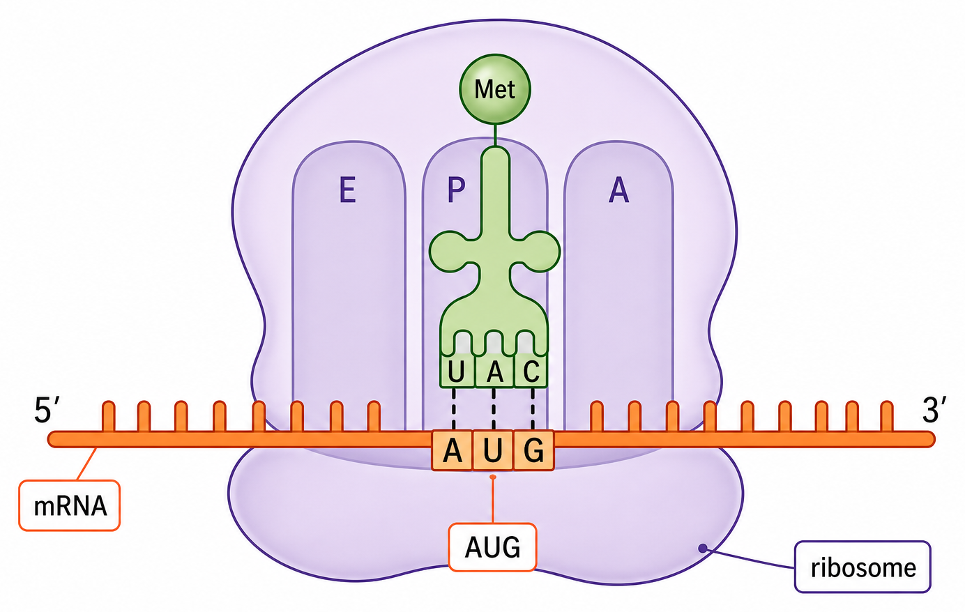
Translation Initiation Places the Start Codon in the P Site
HL only
1
The small ribosomal subunit binds the mRNA and positions the start region for scanning or recognition.
2
The initiator tRNA carrying methionine pairs with AUG. This tRNA is placed directly in the P site, establishing the reading frame.
3
The large subunit joins to complete the ribosome. The A site is now open for the tRNA matching the next codon.
AUG inside an already established reading frame can code for methionine without serving as a new start. Initiation depends on context and assembly, not the triplet alone.
A, P and E Sites Track Each tRNA's State
HL only
Ribosomal site
Typical tRNA state during elongation
A (aminoacyl)
incoming charged tRNA paired with the next codon
P (peptidyl)
tRNA carrying the growing polypeptide before peptide transfer
E (exit)
uncharged tRNA leaving after translocation
Before peptide transfer: growing chain in P, new amino acid in A.
After peptide transfer and translocation: the chain-bearing tRNA occupies P, the empty tRNA moves to E, and A opens for the next charged tRNA.
The site letters describe functional positions in the ribosome, not permanent labels on a tRNA. A single tRNA can move A → P → E during one cycle.
A New Polypeptide May Need Folding, Cleavage or Chemical Modification
HL only
Translation produces a polypeptide primary structure. Many proteins become functional only after post-translational processing changes their shape, length, location or chemical properties.
Common processing routes include:
Folding into a specific three-dimensional conformation, sometimes assisted by chaperones.
Cleavage to remove a signal peptide or inactive segment.
Covalent modification, such as phosphorylation or glycosylation, which can alter activity, stability or location.
Assembly with other polypeptide subunits or prosthetic groups.
Not every protein undergoes every modification. The required pathway depends on the protein's sequence, destination and function.
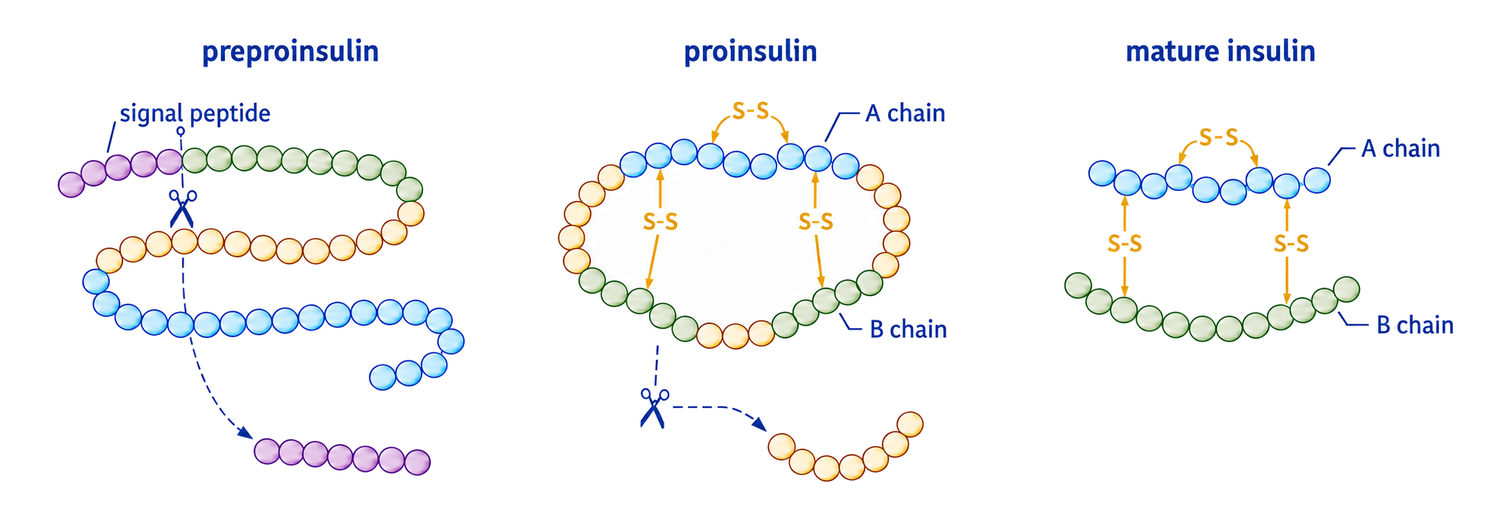
Insulin Becomes Active through Ordered Cleavage and Folding
HL only
1
Preproinsulin contains an N-terminal signal peptide that directs the growing polypeptide into the endoplasmic reticulum. Removing the signal peptide produces proinsulin.
2
Proinsulin folds, and disulfide bonds form between regions that will become the A and B chains.
3
The connecting C-peptide is removed. The A and B chains remain linked by disulfide bonds, producing mature insulin.
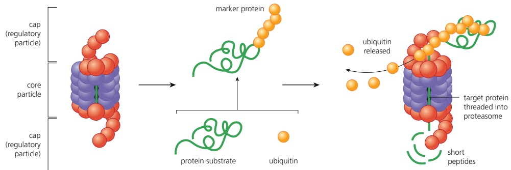
Ubiquitin Directs Selected Proteins to the Proteasome
HL only
1
Proteins selected for degradation are commonly marked with a chain of ubiquitin molecules.
2
The proteasome recognizes the tag, removes and recycles ubiquitin, unfolds the target protein and threads it into a proteolytic core.
3
The protein is cut into short peptides, which can be hydrolysed to amino acids for new synthesis or metabolism.
Selective degradation removes damaged or misfolded proteins and can rapidly lower the abundance of regulatory proteins. Protein concentration therefore depends on both synthesis and breakdown.
Control Protein Output at Several Checkpoints
HL only
Checkpoint
What can change
Consequence for protein output
transcription initiation
promoter and transcription-factor activity
amount of pre-mRNA made
RNA processing
cap, tail and exon combination
mRNA stability, export and encoded sequence
translation initiation
successful AUG recognition and ribosome assembly
whether and where translation begins
post-translational processing
folding, cleavage, modification and assembly
protein activity or location
proteasomal degradation
ubiquitin tagging and breakdown rate
protein lifetime and abundance
Across these checkpoints, sequence direction stays consistent: RNA is made 5′→3′, the ribosome reads mRNA 5′→3′ and the polypeptide grows from N-terminus to C-terminus.
Gene expression is therefore not a single on/off event. A cell controls which message is made, how it is processed, whether it is translated, how the product is activated and how long the protein remains.
Transcription exam focus
[ 8 ]
Explain the process of transcription in prokaryotes.
Hydrogen bonding in transcription
[ 1 ]
The sequence of bases on a short section of the antisense strand of a gene undergoing transcription is shown:
5′ CATG 3′
What is the sequence of bases on the resulting mRNA?
Transcription for gene expression
[ 2 ]
The scientists concluded that auxin activates the transcription of the GH 3 gene. Using the information on the auxin concentration in the stem base in the graph on page 4 and the Northern blot, evaluate whether this conclusion is supported.
Translation exam focus
[ 8 ]
Explain how polypeptides are produced by the process of translation.
Roles in translation
[ 7 ]
Explain the role of RNA in translation, resulting in the formation of polypeptide chains.
Complementary base pairing
[ 3 ]
Outline how translation depends on complementary base pairing.
Genetic code features
[ 5 ]
Describe the genetic code and its relationship to polypeptides and proteins.
Using genetic code table
[ 1 ]
Which sequence of mRNA bases and amino acids could be produced by transcription and translation of the DNA molecule shown?
3' AAAGTGGCACGTATATTT 5' 5' TTTCACCGTGCATATAAA 3′
1st base in codon
2nd base U
2nd base C
2nd base A
2nd base G
3rd base in codon
U
Phe
Ser
Tyr
Cys
U
U
Phe
Ser
Tyr
Cys
C
U
Leu
Ser
STOP
STOP
A
U
Leu
Ser
STOP
Trp
G
C
Leu
Pro
His
Arg
U
C
Leu
Pro
His
Arg
C
C
Leu
Pro
Gln
Arg
A
C
Leu
Pro
Gln
Arg
G
A
Ile
Thr
Asn
Ser
U
A
Ile
Thr
Asn
Ser
C
A
Ile
Thr
Lys
Arg
A
A
Met
Thr
Lys
Arg
G
G
Val
Ala
Asp
Gly
U
G
Val
Ala
Asp
Gly
C
G
Val
Ala
Glu
Gly
A
G
Val
Ala
Glu
Gly
G
Sequence of mRNA bases
Sequence of amino acids
UUU-GAG-GCU-CGA-UAU-UUU
Phe-Glu-Ala-Arg-Tyr-Phe
AAA-CUC-CGA-GCU-AUA-UUU
Lys-Leu-Arg-Ala-Ile-Phe
UUU-CAC-CGU-GCA-UAU-AAA
Phe-His-Arg-Ala-Tyr-Lys
AAA-GUG-GCA-CGU-AUA-UUU
Lys-Val-Ser-Arg-Ile-Phe
Elongation of polypeptide
[ 2 ]
Six polypeptides are shown in the diagram. Explain the different lengths of these polypeptides.
Mutations changing protein structure
[ 8 ]
Explain the cause of sickle cell anemia and how this disease affects humans.
Directionality exam focus
HL only
[ 1 ]
Using the diagram, identify, with a reason, whether X or Y is the start codon.
Initiation of transcription at promoter
HL only
[ 2 ]
Explain the function of a promoter in DNA.
Non-coding sequences in DNA
HL only
[ 2 ]
DNA has regions that do not code for proteins. State two functions of these regions. 1. 2.
Post-transcriptional modification
HL only
[ 1 ]
What happens to mRNA after transcription in eukaryotic cells?
Alternative splicing
HL only
[ 1 ]
The number of protein-coding genes in the human genome is estimated to be about 20000 , which is much less than the size of the proteome. What is one reason for this?
Translation initiation
HL only
[ 4 ]
Outline the roles of the different binding sites for tRNA on ribosomes during translation.
Polypeptide modification
HL only
[ 2 ]
Insulin is produced by cutting C -peptide from the precursor molecule proinsulin. Suggest why group 1 has a greater level of C-peptide than group 2.
D1.3 Mutation and gene editing
Mutation and gene editing explain how DNA sequence changes arise, affect proteins, create variation and can be studied or altered deliberately.
Syllabus
First assessment 2025
Topic
D1.3
Level
HL
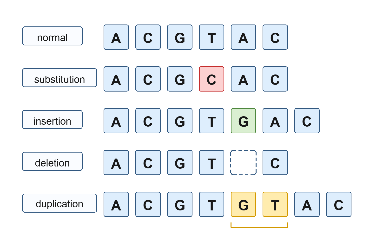
A Mutation Changes DNA Sequence, Not a Whole Organism at Once
A gene mutation is a change in the order or number of DNA bases within a gene. It creates a new sequence; its later effect depends on where the change occurs.
Substitution: one nucleotide is replaced by another.
Insertion: one or more nucleotides are added.
Deletion: one or more nucleotides are lost.
Duplication: a DNA segment is copied and repeated.
Mutation names describe the DNA change. They do not by themselves tell you whether a protein, cell or organism will be affected.
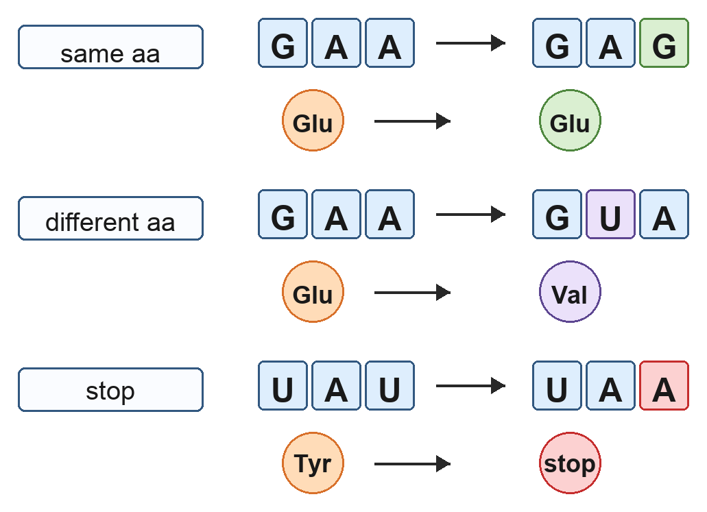
One Base Substitution Can Be Silent, Missense or Nonsense
A base substitution replaces one nucleotide without changing sequence length. In a population, a one-base variant present among individuals is a single-nucleotide polymorphism (SNP).
Coding outcome
Why it happens
Possible protein effect
silent
altered codon still specifies the same amino acid because the code is degenerate
primary structure unchanged
missense
altered codon specifies a different amino acid
folding or function may change
nonsense
altered codon becomes a stop codon
translation ends early
A substitution outside a coding sequence can still matter if it changes a promoter or other regulatory sequence; some substitutions have no detectable effect.
An Indel Shifts the Reading Frame Unless Its Size Is a Multiple of Three
A ribosome reads nucleotides in non-overlapping groups of three. Inserting or deleting a number of bases not divisible by three changes the grouping from that point onward: a frameshift.
A one- or two-base indel usually changes many downstream codons and may create an early stop.
A three-base indel adds or removes one codon without shifting later codon boundaries.
A larger in-frame indel can still disrupt function by adding or removing amino acids.
Do not call every insertion or deletion a frameshift. Test whether the number of bases changed is a multiple of three.
DNA Damage Becomes a Mutation When the Altered Sequence Is Fixed
DNA replication error or DNA damage → proofreading and repair act → unrepaired or misrepaired change persists → later replication copies the altered sequence
Changes can begin inside the cell through:
incorrect nucleotide insertion during DNA replication
failure of proofreading or repair
chromosome breakage or other DNA damage
Mutagens increase mutation frequency by damaging DNA. Important classes include chemical mutagens, ionizing radiation such as X-rays, and ultraviolet radiation.
Exposure causes DNA damage probabilistically; it does not guarantee that a specific gene will mutate. Repair can restore the original sequence.
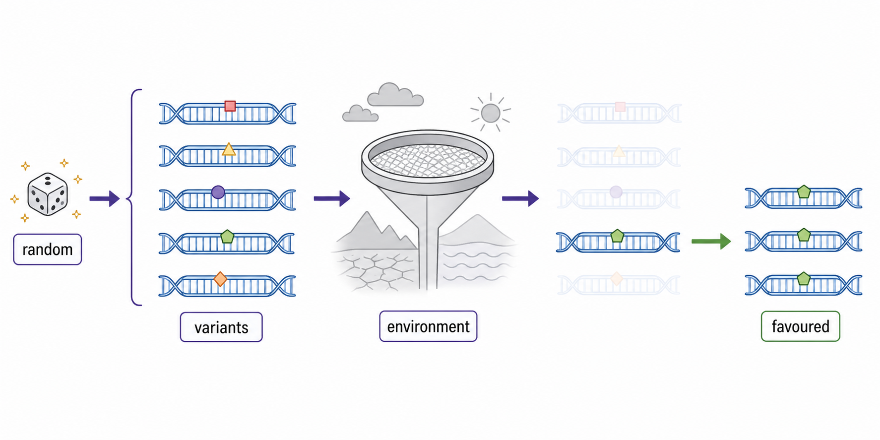
Mutation Is Random Relative to Need, but Its Probability Is Not Uniform
A mutation does not arise because an organism needs a useful trait. A change can occur before an environmental challenge and later prove harmful, neutral or advantageous.
Mutation probability can still vary with:
base identity and local sequence context
how often a region is copied or transcribed
access to proofreading and repair systems
dose and type of mutagen exposure
Random relative to need is not the same as equally likely at every base. Natural selection is the non-random filter; it does not direct the earlier mutation.
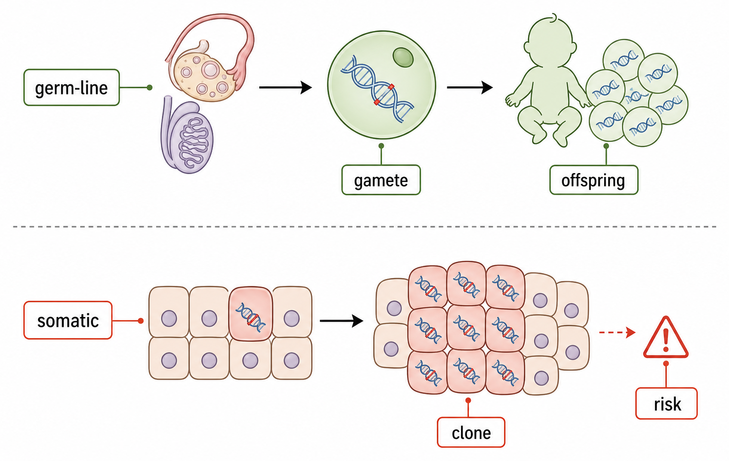
Cell Lineage Determines How Far a Mutation Can Travel
Mutation location
Cells that can inherit it
Biological reach
germ-line lineage
gametes and potentially the offspring formed from them
can pass between generations
somatic cell
mitotic descendants of that body cell
remains within the individual and its cell clone
A somatic mutation can contribute to cancer if it affects control of cell division, DNA repair or cell death. Further mutations and selection among cell clones can then expand the abnormal lineage.
A somatic mutation is not inherited by the person's offspring merely because many body cells carry it; it must enter the germ line to cross generations.
Mutation Creates Alleles; Natural Selection Changes Their Frequencies
Mutation is the original source of new alleles. Recombination can reshuffle existing alleles, but it does not create a new DNA sequence at a locus.
new mutation → new allele → inheritance places the allele in a population → environment affects survival and reproduction → allele frequency may change over generations
Most new mutations are neutral or harmful in their current context; a smaller number can improve reproductive success under particular conditions. The same allele can have different effects in different environments.
Populations evolve because heritable allele frequencies change. An individual does not mutate adaptively and then evolve during its lifetime.
Predict a Mutation's Consequence by Following Four Decisions
Ask
What the answer predicts
What changed in the DNA?
substitution, insertion, deletion or duplication
Where is the change?
coding, regulatory or other sequence; possible molecular consequence
Which cell lineage carries it?
local somatic clone or possible inheritance through gametes
Does it alter reproductive success?
whether selection may change its frequency
The causal chain can stop at any stage: a DNA change can be repaired, lie in a tolerant region, preserve the amino acid, or make no detectable phenotypic difference.
Mutation generates variants without foresight. Cell lineage controls their reach, and natural selection later filters heritable variation according to environmental conditions.
Gene Knockout Tests Function by Removing One Gene's Activity
HL only
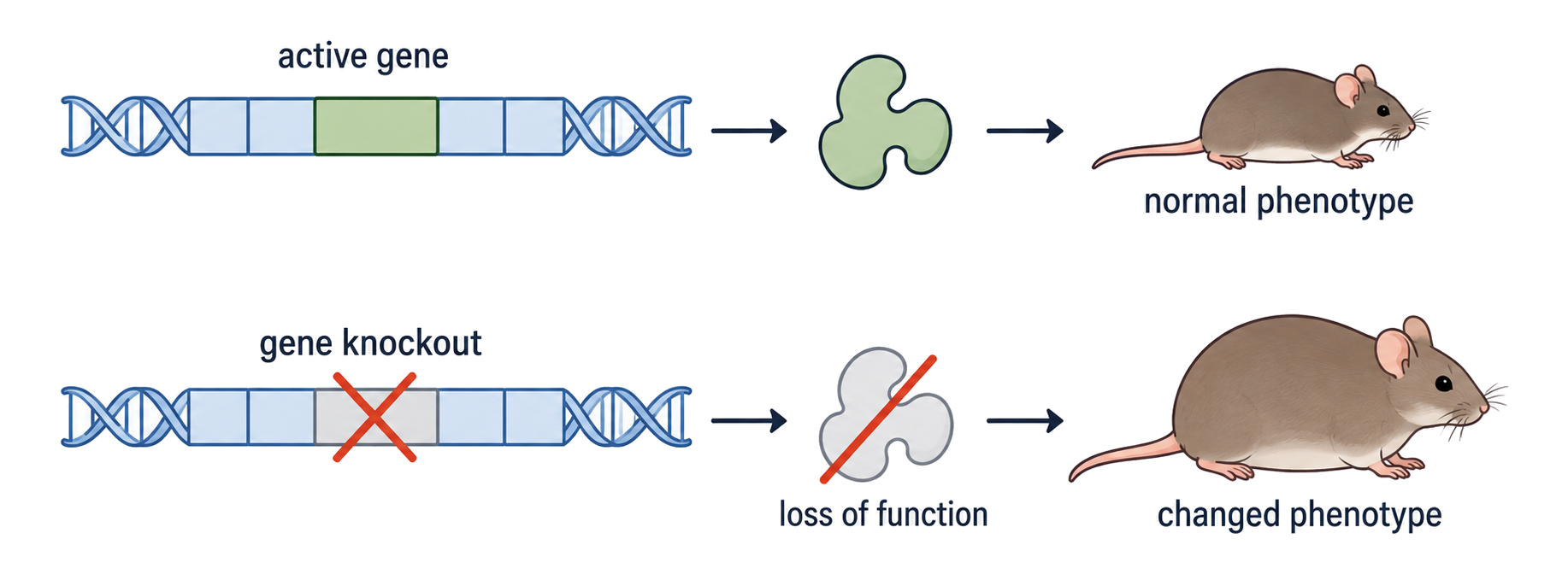
A gene knockout makes a selected gene non-functional. Researchers compare the knockout phenotype with an otherwise similar control to infer what the missing gene normally contributes.
selected gene active in control → normal gene product present → baseline phenotype
selected gene knocked out → gene product absent or reduced → any reproducible phenotype difference supports a role for that gene
A changed phenotype supports involvement, not a complete one-gene/one-trait explanation. Developmental compensation, background mutations and environmental differences must be controlled.
Knockout Libraries Turn One Comparison into a Search across Many Genes
HL only
A knockout library contains organisms or cell lines in which different genes have been made non-functional. Researchers can screen the collection for a phenotype and identify candidate genes.
Common model organisms include:
mice for mammalian physiology and disease
Drosophila for development and inheritance
zebrafish for vertebrate development and transparent embryos
Arabidopsis for plant genetics
Model organisms are useful because core genes, the genetic code and many cell processes are shared. They also have short generations, tractable breeding or large existing genetic resources.
A model result is evidence for a testable hypothesis in another species, not automatic proof that the gene has an identical effect in humans.
Natural CRISPR-Cas Defence Stores and Reuses Viral Sequence Information
HL only
1
After viral infection, a bacterium can insert a short fragment of viral DNA as a spacer among CRISPR repeats in its own genome.
2
The spacer is transcribed into guide RNA. Its base sequence can pair with complementary DNA from the same virus during a later infection.
3
Guide RNA associates with a Cas nuclease. Complementary pairing positions the nuclease, which cuts the matching viral DNA and prevents successful replication.
Specificity comes from base pairing between guide RNA and target DNA; Cas9 supplies the cutting activity.
A Designed Guide RNA Positions Cas9 at a Chosen DNA Target
HL only
1
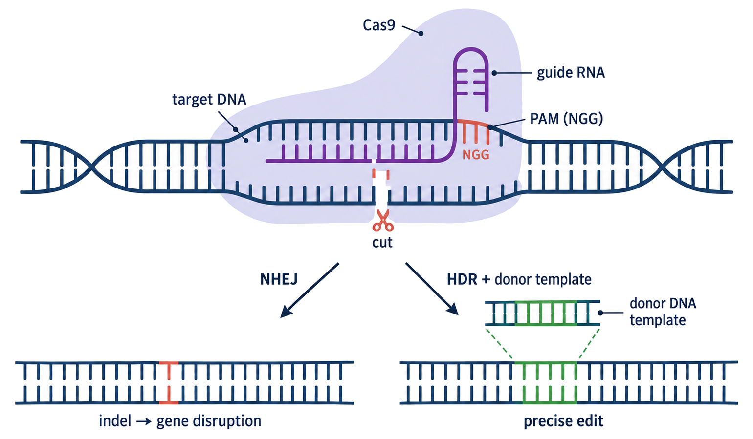
Researchers choose a target sequence and design a guide RNA with a complementary region. The guide RNA and Cas9 form a complex that searches DNA for a compatible target beside the required recognition motif.
2
Guide-target base pairing holds the complex at the selected site. Cas9 then makes a double-strand break in the DNA.
Cas9 makes the cut; the final edit is produced when the cell repairs that break. Similar off-target sequences can sometimes also be cut, so the result must be checked.
DNA Repair Determines What Edit Follows the Cas9 Cut
HL only
Repair context
Likely sequence outcome
Typical use
ends rejoined without a supplied template
small insertions or deletions may disrupt the reading frame
gene disruption or knockout
two sites are cut
intervening segment can be deleted
targeted deletion
repair template is supplied
chosen sequence can be copied into the break
replacement or insertion
define the intended edit → design guide RNA and, if needed, a donor template → deliver editing components → isolate edited cells or organisms → sequence the target → test the phenotype
A desired phenotype alone does not prove the intended edit caused it. Confirm the target sequence, examine plausible off-target sites and compare with suitable controls.
CRISPR-Cas9 can delete, replace, insert or disrupt DNA, but efficiency and precision depend on target sequence, delivery and the cell's repair pathway.
A Sequence Is Conserved When the Same Positions Persist across Lineages
HL only
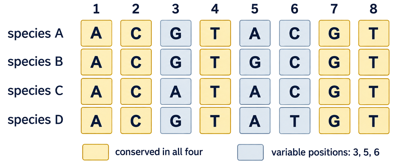
A conserved sequence remains identical or similar among species; a highly conserved sequence has changed little across long evolutionary time.
Read an alignment by columns. A position shared by all sampled species is conserved in that sample; a column containing different bases is variable.
Conservation can occur in protein-coding or regulatory DNA. The species sampled and the time since their divergence affect how strong the pattern appears.
Conservation Can Reflect Selection, Mutation Rate—or Both
HL only
Hypothesis
Mechanism
Prediction
functional constraint with purifying selection
harmful variants reduce reproductive success and are removed
disrupting the sequence is likely to impair function
lower mutation rate
fewer sequence changes arise, perhaps because repair is especially effective
conservation can persist even before selection acts
The explanations are not mutually exclusive. An essential sequence may both acquire mutations slowly and lose harmful variants rapidly through purifying selection.
Highly transcribed genes and their transcribed strands can show lower mutation rates, consistent with enhanced access to repair machinery.
Conservation suggests importance, but sequence comparison alone does not reveal the exact function. Knockout or targeted editing can test the hypothesis experimentally.
Combine Intervention and Comparison to Infer Gene Function
HL only
Evidence route
Core question
Strength
Main caution
knockout
what changes when gene activity is removed?
supports a causal role
other changes and compensation need controls
CRISPR-Cas9 edit
what changes after a chosen sequence is altered?
tests a precise sequence hypothesis
edit and off-target sites must be verified
conservation
which positions persisted across evolution?
prioritizes likely functional regions
correlation does not identify exact function
Conservation can nominate a candidate sequence → targeted editing can change it → phenotype and molecular measurements can test the predicted function → sequencing confirms what was actually altered.
The strongest inference combines comparative evidence with a controlled intervention. Neither an alignment nor an edited phenotype should be interpreted alone.
Gene mutations
[ 2 ]
Mutations may increase variation within a species. Compare and contrast substitution and insertion mutations.
Base substitution consequences
[ 4 ]
Outline how a base substitution leads to sickle cell anemia.
Causes of mutation
[ 2 ]
Explain how chemical substances can cause cancer.
Randomness in mutation
[ 1 ]
What is a feature of mutations?
Consequences in germ vs. somatic cells
[ 1 ]
A mutation in which type of cell could be inherited?
Mutation as source of variation
[ 1 ]
What causes variation in both sexually and asexually reproducing organisms?
Gene knockout
HL only
[ 1 ]
What is gene knockout used for?
CRISPR-Cas9 gene editing
HL only
[ 3 ]
Explain ways in which CRISPR-Cas9 gene editing could be used to change the mutated dystrophin protein produced.
Conserved sequences
HL only
[ 1 ]
A bioinformatics analysis was performed on the protein PSY transcribed from the gene from corn and from daffodil to obtain the sequence alignment.
On the alignment, identify the longest part of the sequence where the consecutive amino acids are the same.
E L SQA SRWP VWASLL LYRQI LDE I EANDYNNF TKRAYVSKV
Corn
KKLLALPVAYGKSLLLPCSLRN---GQT
Daffodil
KRLAALPLA YGKSLLIPLSLRPPSLSKA
* * * * * * * * * * * * * * * *
D2.1 Cell and nuclear division
Cell and nuclear division coordinate DNA replication, chromosome movement, cytokinesis, meiosis, cell-cycle control and proliferation to produce new cells in organisms.
Syllabus
First assessment 2025
Topic
D2.1
Level
HL
Cell Division Extends an Existing Cell Lineage
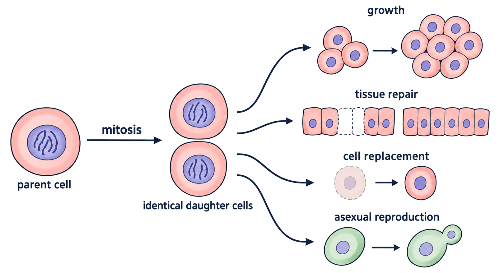
Every new cell arises when a pre-existing parent cell divides. The daughter cells inherit cellular material and DNA from that lineage; they are not assembled from non-living parts.
Cell division supplies new cells for:
growth of a multicellular organism
replacement of worn or damaged cells
tissue repair after injury
reproduction in unicellular organisms and some multicellular organisms
Cell division increases cell number. Growth of an individual cell increases cell size; organisms often require both processes.
Animal Cells Pinch In; Plant Cells Build a Cell Plate
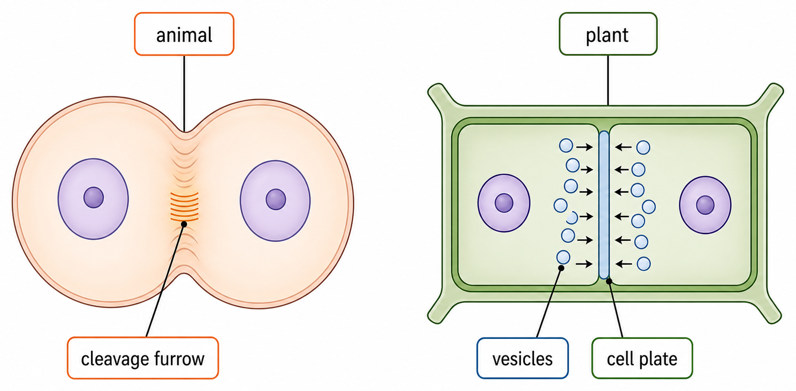
Cytokinesis partitions the cytoplasm after nuclear division so the daughter nuclei become separate cells.
Feature
Animal cell
Plant cell
starting constraint
flexible plasma membrane
rigid existing cell wall
mechanism
actin–myosin contractile ring tightens a cleavage furrow
Golgi-derived vesicles fuse at the equator
result
membrane pinches inward
cell plate becomes new membranes and wall between daughters
Both mechanisms divide one cytoplasm around two daughter nuclei, but they solve the mechanical problem in opposite directions: inward constriction versus construction from the centre outward.
Equal Chromosomes Do Not Require Equal Cytoplasm
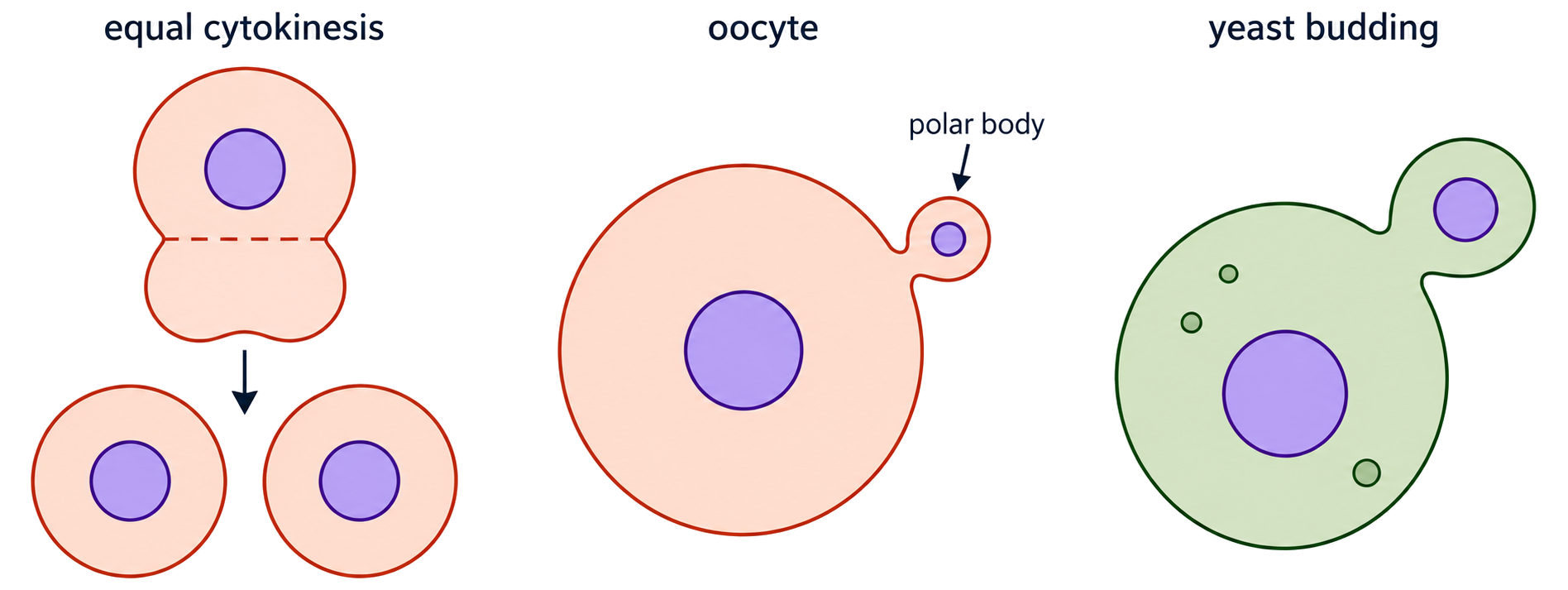
Cytokinesis often gives daughter cells similar cytoplasmic volumes, but the partition can be unequal when the daughters have different immediate functions.
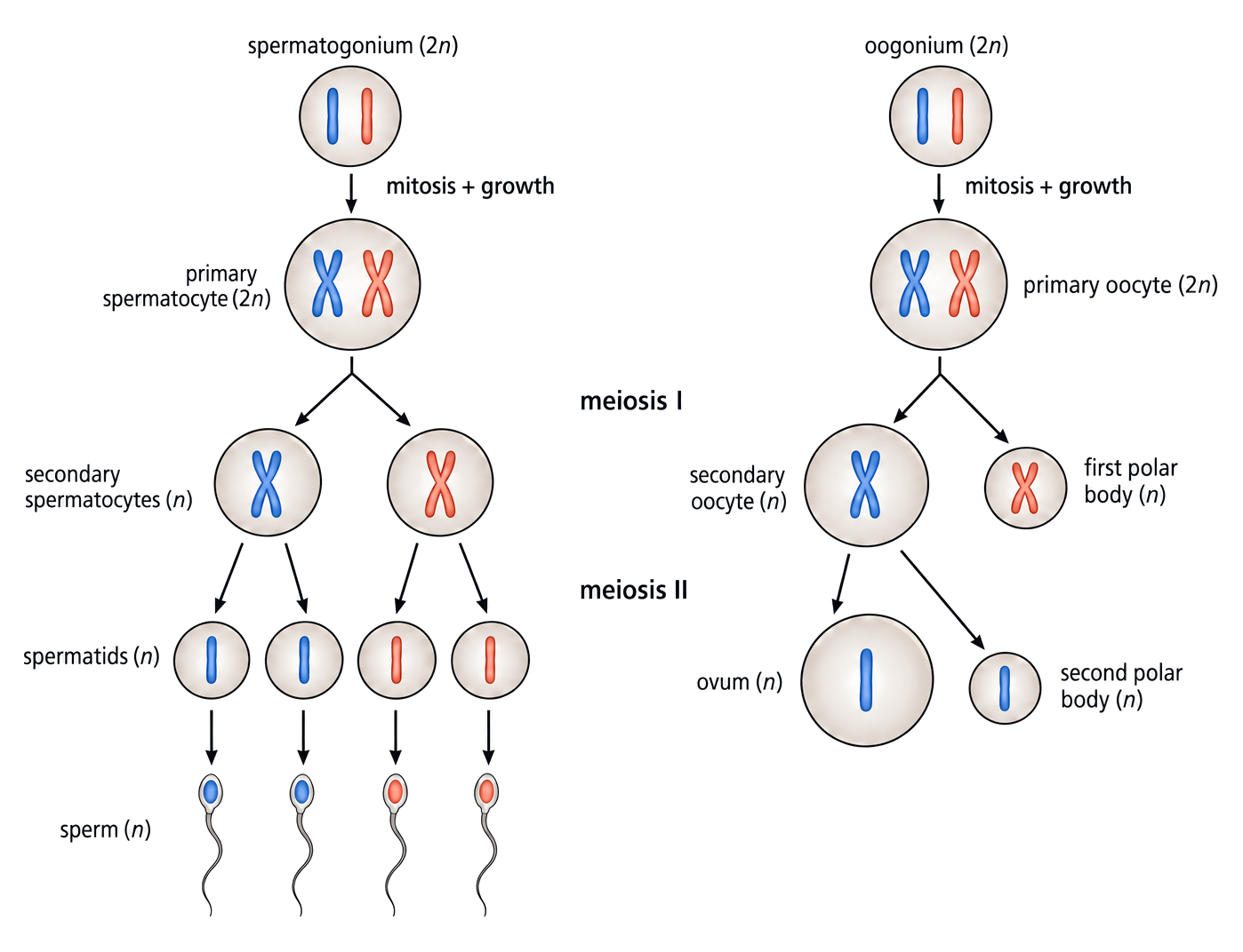
Oogenesis: one cell retains most cytoplasm, organelles and stored nutrients to become the ovum; small polar bodies mainly remove extra chromosome sets.
Yeast budding: a smaller bud grows from the parent and separates after receiving a nucleus and essential cell components.
Unequal cytokinesis refers to cytoplasmic allocation, not deliberately unequal chromosome inheritance. Normal daughter nuclei still require the appropriate chromosome set.
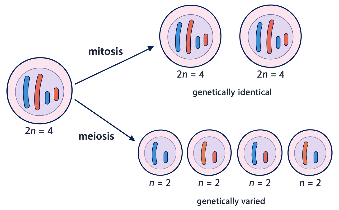
Mitosis Preserves Chromosome Number; Meiosis Reduces It
Dimension
Mitosis
Meiosis
nuclear divisions
one
two after one DNA replication
usual nuclei produced
two
four
chromosome number
maintained
halved
genetic relationship
normally identical to parent and each other
varied combinations
main roles
growth, replacement, repair, asexual reproduction
production of cells that develop into gametes
Diploid (2n) nuclei contain two homologous sets of chromosomes. Haploid (n) nuclei contain one set.
Mitosis and meiosis are nuclear divisions. Cytokinesis is the separate division of cytoplasm that usually follows.
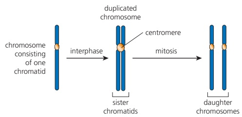
Replication Creates Sister Chromatids before Nuclear Division
1
Before S phase, one chromosome contains one DNA molecule. During S phase that DNA is replicated.
2
After replication, the chromosome consists of two nearly identical sister chromatids joined at a centromere. The chromosome count has not doubled, but the DNA amount has.
3
When the sister chromatids separate, each becomes an individual daughter chromosome. Sending one copy to each future nucleus preserves a complete genome.
Do not count chromatids as separate chromosomes while they remain joined at one centromere.
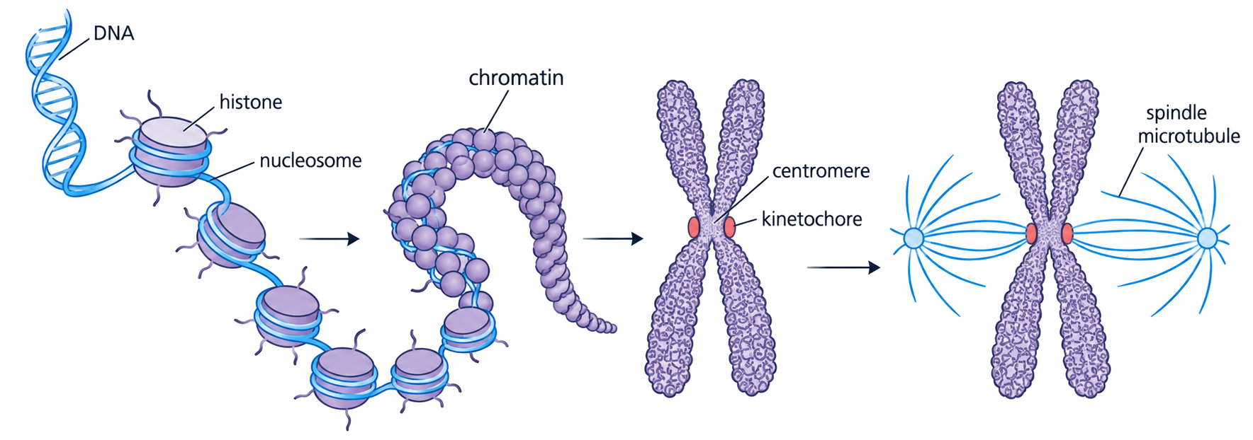
Condensation and Spindle Forces Make Chromosomes Movable
Each chromosome is one very long DNA molecule. Accurate division requires it to be packaged into a compact unit and attached to machinery that can position and separate it.
Mitosis and meiosis share three mechanical features:
DNA wrapped around histones and nucleosomes condenses into chromosomes.
Spindle microtubules attach through centromere-associated structures.
Microtubule dynamics and motor proteins position and move chromosomes.
Condensation does not copy DNA. It changes packaging so long molecules can move with less tangling or breakage.
Mitosis First Condenses Chromosomes and Aligns Their Centromeres
1
Prophase: chromatin condenses into visible duplicated chromosomes; the nucleolus disappears, the nuclear envelope breaks down, and the spindle forms.
2
Metaphase: spindle microtubules attach to the centromere region from opposite poles and position chromosome centromeres at the cell equator.
Identification cues:
condensed chromosomes still scattered or nuclear boundary disappearing → prophase
duplicated chromosomes arranged along one central plane → metaphase
Mitosis is continuous; phase names label dominant visible events rather than pauses between separate processes.
Mitosis Then Separates Sister Chromatids and Rebuilds Nuclei
1
Anaphase: centromere linkage is released and sister chromatids move to opposite poles. Once separated, each chromatid is a daughter chromosome.
2
Telophase: chromosomes reach the poles and decondense; nuclear envelopes and nucleoli re-form around the two chromosome sets.
Identification cues:
two separating groups, often V-shaped as centromeres lead → anaphase
two groups at opposite ends with new nuclear boundaries → telophase
Because sister chromatids were replicated copies and one moves to each pole, the two daughter nuclei normally contain identical chromosome sets.
Identify a Mitotic Stage from Chromosome Evidence, Not Cell Shape
Use a fixed observation sequence:
Are individual condensed chromosomes visible?
Are they scattered, aligned at one equator, separating, or already at opposite poles?
Is one nuclear envelope present, absent, or re-forming as two?
Dominant observation
Best stage identification
chromatin diffuse inside an intact nucleus
interphase, not mitosis
condensed chromosomes not yet aligned
prophase
chromosomes aligned at one equator
metaphase
daughter chromosomes moving apart
anaphase
two chromosome groups with re-forming nuclei
telophase
A stained root-tip squash contains many cells in different stages because division is not synchronized. Count only cells whose chromosome evidence is sufficiently clear.
A single still image may lie near a phase boundary. Record the visible cue and acknowledge uncertainty rather than forcing a label from cell outline alone.
Reconstruct How One Replicated Cell Becomes Two Daughter Cells
DNA replication creates joined sister chromatids → chromosomes condense and attach to the spindle → metaphase alignment checks bipolar attachment → sister chromatids separate → two nuclei re-form → cytokinesis partitions the cytoplasm
Continuity requirement
What supplies it
complete genome in each nucleus
replication followed by equal chromatid separation
controlled chromosome movement
condensation, spindle microtubules and motor proteins
two separate cells
animal cleavage furrow or plant cell plate
suitable daughter-cell contents
equal or functionally unequal cytoplasmic partition
To identify a stage, prioritize chromosome position and nuclear-envelope state. To explain the outcome, connect those observations to what is being separated.
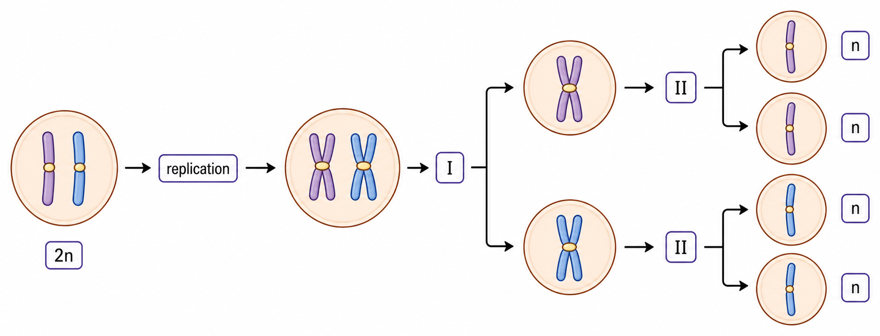
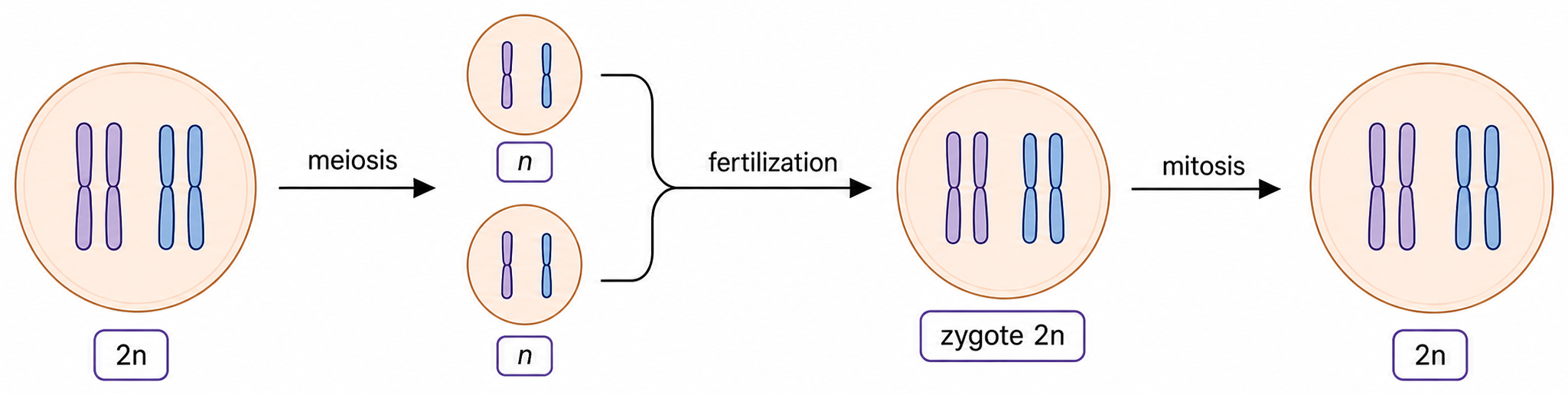
One DNA Replication Followed by Two Divisions Produces Haploid Nuclei
1
Before meiosis, S phase replicates every chromosome into two sister chromatids. The nucleus is still diploid because both homologues of each pair remain present.
2
In meiosis I, homologous maternal and paternal chromosomes separate into different nuclei. Chromosome number is reduced from diploid to haploid, although each chromosome still has two chromatids.
3
There is no second DNA replication. In meiosis II, sister chromatids separate, producing four haploid nuclei with one chromosome from each homologous pair.
Reduction prevents chromosome number doubling in every generation: haploid gametes fuse at fertilization to restore the diploid number.
Meiosis I Separates Homologues; Meiosis II Separates Chromatids
A bivalent is a paired set of duplicated homologous chromosomes: one maternal homologue and one paternal homologue, each made of two sister chromatids.
Question
Meiosis I
Meiosis II
what aligns?
bivalents
individual duplicated chromosomes
what separates?
homologous chromosomes
sister chromatids
do centromeres divide?
no
yes
chromosome-number effect
diploid → haploid
remains haploid
Use the object being separated in explanations: homologues move apart in anaphase I; sister chromatids move apart in anaphase II.
Calling both events 'chromosomes separating' hides the reason meiosis I is the reduction division.
Non-Disjunction Sends Both Copies to One Pole
1
A homologous pair can fail to separate in meiosis I, or sister chromatids can fail to separate in meiosis II. This failure is non-disjunction.
2
Both copies move to one pole while the opposite pole receives none. Later division therefore cannot give every gamete the standard chromosome number.
3
The affected meiosis produces gametes with an extra chromosome (n + 1) and/or a missing chromosome (n − 1), depending on when the error occurred.
4
After fusion with a normal haploid gamete, an n + 1 gamete can produce a trisomic zygote; an n − 1 gamete can produce a monosomic zygote.
Non-disjunction can create too many or too few chromosomes. It is not defined only by an extra chromosome.
Trisomy 21 Usually Begins with a Meiotic Separation Error
chromosome 21 non-disjunction during gamete formation → gamete receives two copies of chromosome 21 → fertilization by a normal gamete adds one more copy → zygote has three copies of chromosome 21
The resulting trisomy 21 gives the zygote 47 chromosomes rather than the usual 46 and can cause Down syndrome.
The developmental effects vary among individuals because an extra chromosome changes the dosage of many genes, not just one gene.
Down syndrome is a chromosome-number condition. It is not caused by a point mutation within chromosome 21.
Crossing Over Recombines Alleles within Homologous Chromosomes
1
During prophase I, duplicated homologous chromosomes pair closely as a bivalent. Corresponding gene loci align.
2
Non-sister chromatids break at corresponding positions and rejoin to the other homologue. The visible connection is a chiasma.
3
Equivalent DNA segments are exchanged, producing recombinant chromatids with new combinations of maternal and paternal alleles.
Crossing over is between non-sister chromatids of homologous chromosomes. It rearranges existing alleles; it does not necessarily create new alleles.
Random Orientation and Fertilization Multiply Gamete Variety
At metaphase I, each bivalent can face either pole independently of the others. The maternal or paternal homologue that enters a gamete is therefore random for each pair.
2n
For humans, n=23, so random orientation alone can produce 223—more than 8 million—chromosome combinations before crossing over is counted.
Random fusion of one genetically varied sperm with one genetically varied egg multiplies the possible allele combinations again.
Crossing over changes allele combinations within chromosomes; random orientation changes which whole maternal and paternal homologues travel together.
Track What Separates to Explain Reduction, Error and Variation
Event
What changes
Main consequence
replication before meiosis
each chromosome gains a sister chromatid
DNA prepared for two divisions
meiosis I
homologous chromosomes separate
chromosome number is halved
meiosis II
sister chromatids separate
four haploid products can form
non-disjunction
one required separation fails
aneuploid gametes may form
Variation is layered: crossing over recombines alleles within chromosomes, random orientation assort homologues independently, and random fertilization combines two independently produced gametes.
When explaining any meiotic outcome, name the stage, the chromosome object that should separate, the chromosome number before and after, and whether the result changes number, allele combination or both.
Cell Proliferation Repeats Mitosis for Growth and Repair
HL only
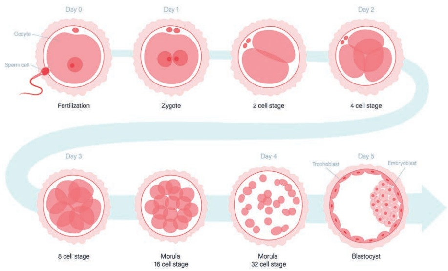
Cell proliferation is an increase in cell number through repeated cell growth and mitotic division. The new cells may remain unspecialized, differentiate or replace cells that were lost.
Early embryo: rapid divisions build cell number before extensive differentiation.
Plant meristems: dividing cells at apical or lateral growth regions supply new plant tissues.
Routine replacement: stem-cell lineages replenish short-lived cells such as epidermal cells.
Wound repair: fibroblasts and other cells proliferate to rebuild tissue and extracellular matrix.
Proliferation describes more cells. Cell enlargement and differentiation can follow, but they are different processes.
The Cell Cycle Alternates Preparation with Division
HL only
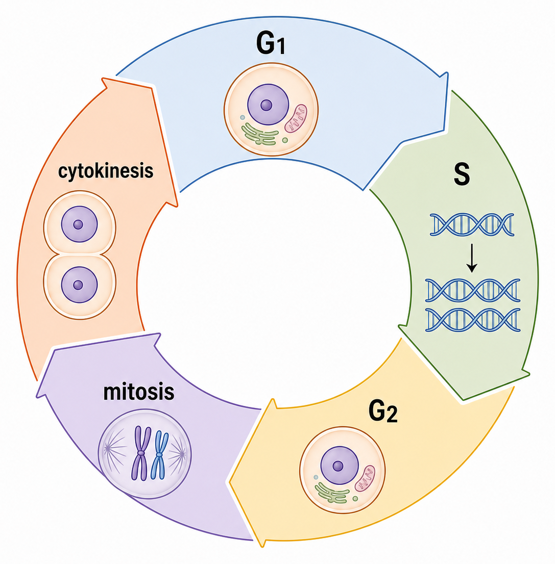
The cell cycle is the repeating sequence in which a cell grows and prepares during interphase, divides its nucleus by mitosis and partitions its cytoplasm by cytokinesis.
G1 growth and biosynthesis → S-phase DNA replication → G2 growth and division preparation → mitosis → cytokinesis → daughter cells enter a new cycle or leave active cycling
A cell is not in mitosis for most of its cycle. Interphase is usually the longest portion, so most cells in a tissue sample are expected to appear in interphase.
G1 Builds the Cell, S Copies DNA and G2 Prepares Division
HL only
Interphase stage
Main work
Chromosome state by the end
G1
cell growth, metabolism, protein and organelle production
each chromosome has one chromatid
S
DNA replication
each chromosome has two sister chromatids
G2
further growth, protein synthesis and preparation for spindle formation
replicated chromosomes remain joined
The order matters: the cell first builds capacity, then copies the genome once, then checks and prepares the machinery needed to distribute those copies.
DNA quantity doubles during S phase, but chromosome number does not double because the sister chromatids remain joined at their centromere.
Interphase Is Active Even When Chromosomes Are Not Visible
HL only
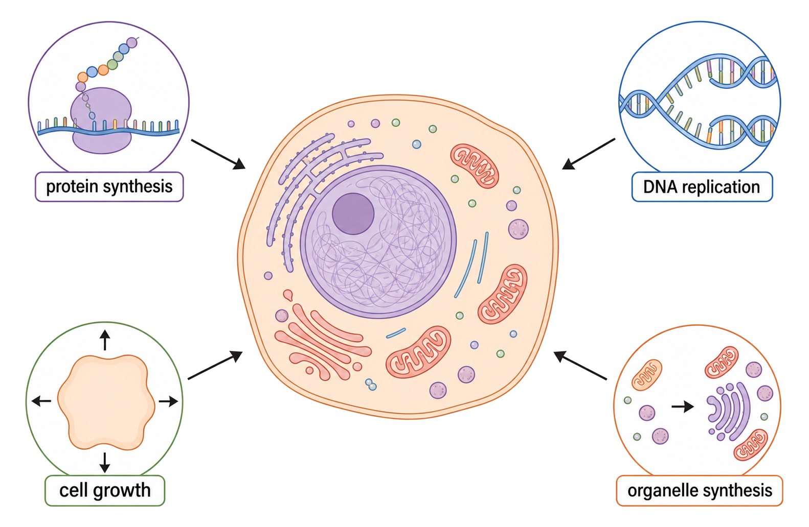
During interphase the cell transcribes genes, synthesizes proteins, grows its cytoplasm, accumulates energy and increases organelles. DNA is dispersed as chromatin and remains accessible for gene expression.
Interphase duration varies with cell fate: rapidly proliferating embryo or meristem cells cycle quickly, many adult cells divide only when signalled, and some differentiated cells remain outside active division for long periods.
A nucleus that looks uniform under a light microscope is not resting. Lack of visible condensed chromosomes is evidence of chromatin state, not metabolic inactivity.
Cyclin–CDK Complexes Turn Cell-Cycle Transitions On
HL only
Cyclin-dependent kinases (CDKs) are present but require particular cyclins to become active. Cyclin concentrations rise and fall, giving the control system time-specific signals.
1
Cyclin accumulates and binds its CDK → the active complex phosphorylates target proteins → a checkpoint transition can occur once the relevant conditions and threshold are satisfied.
2
At the G2/M transition, cyclin–CDK activity forms mitosis-promoting factor (MPF), triggering chromosome condensation, nuclear-envelope breakdown and spindle assembly.
3
Cyclin is then degraded while CDK can be reused. Falling complex activity helps make the transition directional and resets control for a later cycle.
Cyclin level is part of checkpoint control, not the only input. DNA integrity, replication completion, spindle attachment and external signals also influence progression.
Cancer Risk Rises When Growth Signals Stick On or Checkpoint Brakes Fail
HL only
Gene class
Normal role
Cancer-promoting change
Analogy
proto-oncogene
stimulates division when an appropriate signal is present
gain-of-function mutation creates an oncogene with excessive or constant activity
accelerator stuck on
tumour-suppressor gene
stops the cycle, repairs damage or promotes apoptosis
loss-of-function mutation removes restraint
brake lost
A mutant Ras oncogene can keep growth-signalling pathways active without the normal extracellular signal. One activated allele may be sufficient to increase signalling.
Loss of p53 function can prevent arrest or apoptosis after DNA damage. Because a remaining functional copy can still supply p53, both copies often need to be lost in the affected cell lineage.
Cancer usually develops through accumulated mutations and clonal selection, not one mutation that instantly creates a fully malignant tumour.
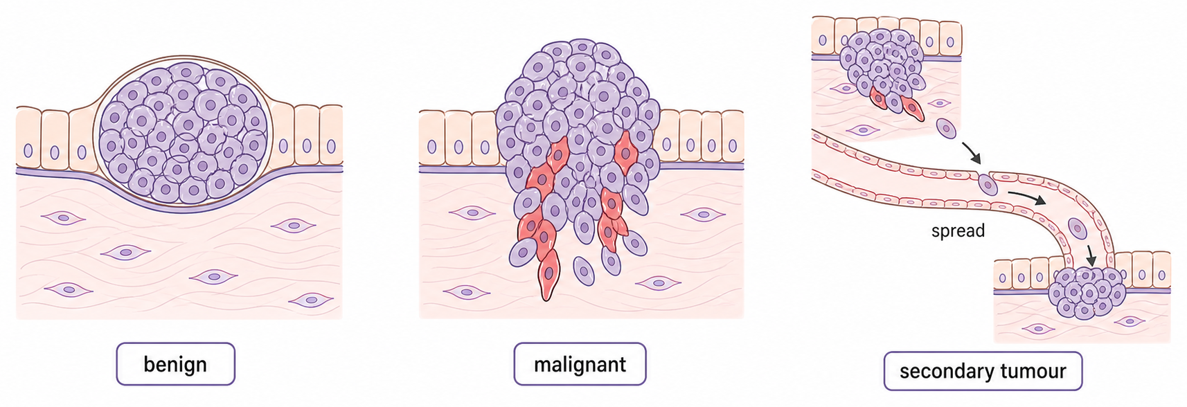
Invasion and Metastasis Distinguish Malignant Tumours
HL only
Property
Benign tumour
Malignant tumour
local growth
often slower and bounded
often faster and poorly controlled
invasion
does not invade neighbouring tissue
penetrates and damages neighbouring tissue
metastasis
absent
cells may detach, travel and form secondary tumours
Metastasis requires several steps: cells detach from the primary tumour, enter blood or lymph, survive transport, leave the vessel and establish a secondary tumour elsewhere.
A tumour is an abnormal mass produced by excess cell division. Not every tumour is cancerous; malignant invasion and metastatic capacity define cancerous behaviour.
Mitotic Index Estimates the Fraction of Cells Currently Dividing
HL only
MI=TM×100%
Let M be the number of cells observed in mitosis and T the total number of cells observed. If 10 of 95 visible cells are in mitosis,
9510×100%=10.5%
A higher mitotic index means a larger fraction of sampled cells was in mitosis at the observation time. It can support comparison of tissue proliferation or response to treatment.
Mitotic index is not a unique cancer diagnosis. It depends on sampling, stage-identification accuracy and how long cells remain in mitosis; replicate fields and other evidence are required.
Connect Normal Proliferation to Cell-Cycle Control and Cancer
HL only
Growth or repair signal → G1 growth → S-phase genome replication → G2 preparation and checkpoint control → cyclin–CDK activation → mitosis and cytokinesis → daughter cells differentiate, replace tissue or re-enter the cycle
Oncogene activation can increase positive growth signalling, while tumour-suppressor loss can remove arrest, repair or apoptosis. Accumulated changes allow an abnormal clone to proliferate.
Evidence scale
Question it answers
cell-cycle proteins and genes
why is checkpoint control altered?
mitotic index
what fraction of sampled cells is dividing now?
tissue boundary
is the tumour local or invading?
secondary growths
has metastatic spread occurred?
Rapid division alone is not the whole definition of malignancy. A strong explanation connects molecular control failure to clonal growth, tissue invasion and possible metastasis.
Generation of new cells
[ 1 ]
Which process contributes to growth of a multicellular body?
Cytokinesis exam focus
[ 8 ]
Compare and contrast the processes of mitosis and cytokinesis in animal and plant cells.
Equal and unequal cytokinesis
[ 1 ]
Daughter cells usually receive equal amounts of cytoplasm as parent cells undergo cytokinesis. Which of the following is an exception?
Roles of mitosis and meiosis
[ 5 ]
Distinguish between the processes of meiosis and mitosis.
DNA replication prerequisite
[ 1 ]
Distinguish between the quantity of DNA of the cell at G1 and G2.
Shared features
[ 1 ]
What occurs in cell division during both mitosis and meiosis?
Phases of mitosis
[ 9 ]
Describe the events that occur during mitosis.
Identification of mitosis phases
[ 1 ]
The following shows a micrograph.
How many cells are in metaphase?
Meiosis as reduction division
[ 5 ]
Outline what occurs in cells in the first division of meiosis.
Down syndrome
[ 4 ]
Describe how non-disjunction can cause Down syndrome.
Meiosis generates variation
[ 7 ]
Explain the stages and processes of meiosis leading to genetic variation.
Drawing canvas
Cell proliferation
HL only
[ 3 ]
Based on the data, evaluate the evidence for leptin promoting regeneration of liver tissue.
Cell cycle phases
HL only
[ 7 ]
Following germination of seeds, plants undergo a rapid increase in the number of cells. Describe stages in the cell cycle that result in this increase of cells.
Cell growth during interphase
HL only
[ 4 ]
Outline the processes occurring during interphase in the cell cycle.
Cell cycle control by cyclins
HL only
[ 4 ]
Explain how the cell cycle is controlled.
Mutations in cell cycle genes
HL only
[ 4 ]
Explain how changes to the cell cycle can result in tumour formation.
Tumour differences
HL only
[ 1 ]
Which processes occur during the development of secondary tumours?
I. Cytokinesis II. Metastasis III. Mitosis
D2.2 Gene expression [HL only]
Gene expression connects DNA, transcription regulation, epigenetic control, transcript stability, proteomes and environmental signals to phenotype in living cells and tissues.
Syllabus
First assessment 2025
Topic
D2.2
Level
HL
Gene Expression Connects DNA Information to Phenotype
HL only
Gene expression is the use of information in a gene to produce a functional RNA or protein whose activity can affect cell structure, cell behaviour and phenotype.
For a protein-coding gene:
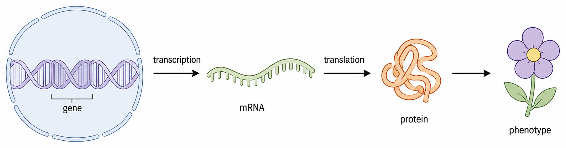
DNA base sequence → transcription → mRNA sequence → translation → amino-acid sequence → folded protein and cellular function → contribution to phenotype
A gene does not act on phenotype by itself. Its effect depends on whether it is expressed, how much product is made, what the product does and the cellular or environmental context.
Protein Output Depends on Several Regulated Rates
HL only
The amount of a protein present at one time reflects a balance between its production and removal, not a single on/off switch.
Control point
Immediate effect
Consequence for protein output
transcription initiation
changes how many mRNA molecules are made
changes the number of templates available
mRNA processing and export
changes which mature transcripts reach ribosomes
changes which messages can be translated
mRNA degradation
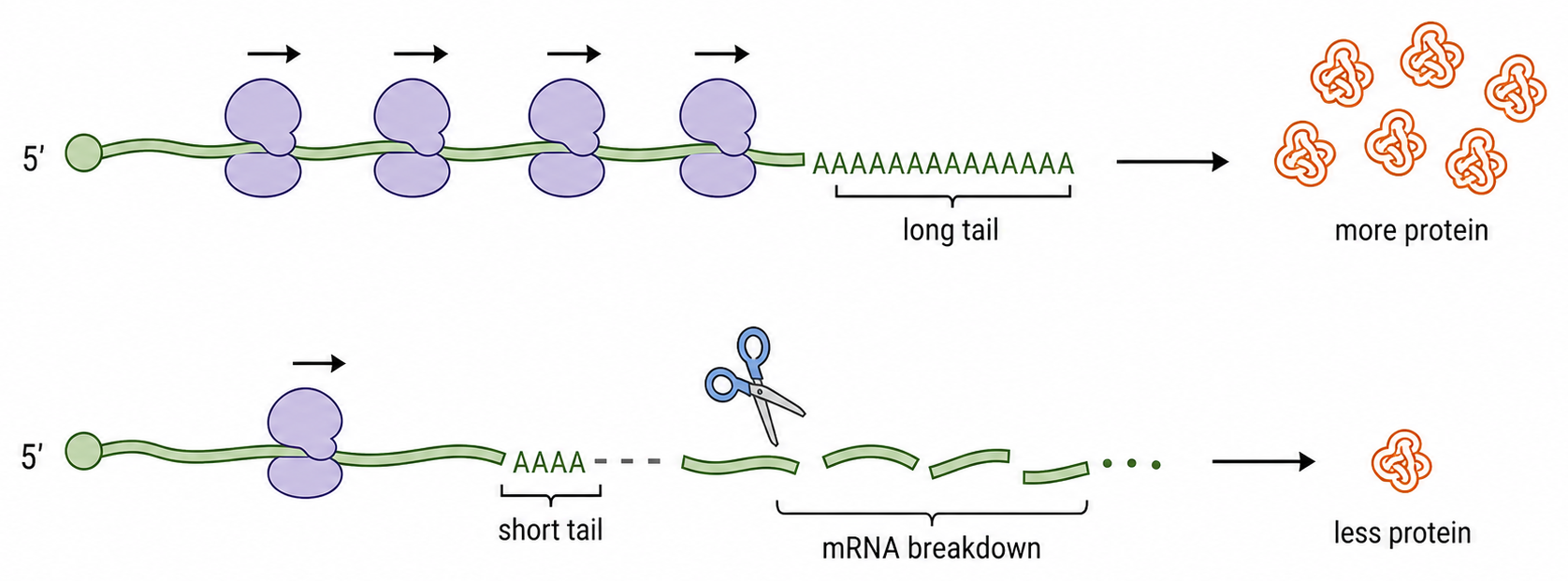
changes transcript lifetime
changes how many translation rounds can occur
translation rate
changes ribosome use of each mRNA
changes protein production per transcript
protein modification or degradation
changes activity or lifetime of the product
changes functional protein present
More mRNA often permits more translation, but mRNA abundance alone does not determine phenotype: translation efficiency, protein activation and protein lifetime also matter.
The Promoter Organizes Transcription Initiation
HL only
A promoter is a non-coding DNA region near the start of a gene where general transcription factors and RNA polymerase assemble to initiate transcription.
Specific DNA sequences are recognized by proteins → a transcription-initiation complex assembles at the promoter → RNA polymerase is positioned on the template strand → transcription begins at the correct site and direction.
Proteins that stabilize or recruit the initiation complex increase transcription. Proteins that block assembly, polymerase recruitment or promoter access decrease transcription.
The promoter is DNA; a transcription factor is a protein that binds DNA. Neither should be called a gene that codes for the protein being regulated.
Enhancers and Repressors Supply Gene-Specific Inputs
HL only
Sequence-specific transcription factors bind regulatory DNA only when their DNA-binding region matches the target base sequence.
Regulatory input
Binding site
Usual effect
activator
enhancer
helps recruit or stabilize the transcription machinery, increasing transcription
repressor
silencer or other regulatory sequence
interferes with activation, promoter access or initiation, decreasing transcription
An enhancer may lie thousands of base pairs upstream or downstream of its gene. DNA looping can bring enhancer-bound activators into contact with proteins at the promoter.
A gene's transcription rate reflects the combination of regulatory proteins present in that cell. One enhancer does not make a gene permanently active in every tissue.
mRNA Lifetime Sets the Window for Translation
HL only
1
An mRNA can be translated repeatedly while it remains intact and accessible to ribosomes. Regulating its degradation therefore changes how long protein production can continue.
2
poly-A tail shortens → the transcript becomes less stable → protective structures are removed → nucleases degrade the mRNA → fewer further rounds of translation occur
A short mRNA lifetime allows a rapid change in protein production when conditions change. A stable mRNA can sustain output even after new transcription has decreased.
Expression Output Is the Result of a Regulated Flow
HL only
regulatory proteins and chromatin access → transcription initiation → mature mRNA abundance and lifetime → translation → protein activity and lifetime → cellular effect
Observation
First control question to ask
little or no mRNA
is transcription initiation repressed or is mRNA rapidly degraded?
abundant mRNA but little protein
is translation inefficient or is protein rapidly removed?
protein present but no expected effect
is the protein inactive, misplaced or missing a required partner?
Gene expression is not simply gene present versus gene absent. Explain a change by naming the regulated stage and tracing its consequence to functional protein and phenotype.
Epigenesis Builds Specialized Cell Types from One Zygote
HL only
Epigenesis is the development of organized patterns of cell differentiation from an initially undifferentiated zygote.
one zygote → repeated mitosis → cells receive different positional or signalling inputs → different genes remain active or inactive → different proteins accumulate → cells acquire specialized structures and functions
A pancreatic β cell expresses proteins for insulin production and secretion.
A skeletal-muscle fibre expresses abundant contractile proteins.
A neuron expresses receptors, ion channels and synaptic proteins suited to signalling.
Differentiation usually changes which genes are expressed, not which genes the cell possesses. Most somatic cell types retain essentially the same genome.
Genome, Transcriptome and Proteome Describe Different Layers
HL only
Layer
What it contains
How it changes
genome
the complete DNA information of a cell
relatively stable across most somatic cells
transcriptome
all RNA transcripts present in a cell or tissue at a stated time
changes with cell type, signals and developmental stage
proteome
all proteins present in a cell, tissue or organism at a stated time
changes through translation, modification, location and degradation
The genome supplies possible information. The transcriptome records which regions are being expressed as RNA now. The proteome records the protein products actually present after further regulation.
The transcriptome and proteome must be tied to a sample and time. Neither is a permanent list of everything the genome could produce.
A Shared Genome Can Produce Distinct Cell Identities
HL only
Cells produced from the same zygote usually share the same genome, but regulatory states make different subsets of that genome accessible and active.
Same underlying genome
Different active output
Functional consequence
insulin gene present
abundant insulin mRNA and protein in pancreatic β cells
blood-glucose regulation
collagen genes present
high collagen expression in many connective-tissue cells
extracellular support
ion-channel genes present
neuron-specific channel and receptor profile
electrical signalling
regulatory state → selected transcriptome → selected proteome → specialized structure and function
A cell type does not normally lose every gene it does not use. Inactivity and absence are different claims.
Promoter DNA Methylation Usually Reduces Transcription
HL only
DNA methylation adds methyl groups to particular cytosines without changing the DNA base sequence. Dense methylation in a promoter is usually associated with reduced transcription of the downstream gene.
promoter cytosines become methylated → proteins that recognize methylated DNA can bind and recruit chromatin-compacting machinery → transcription factors and RNA polymerase gain less access → transcription decreases
Because methyl groups can be added, maintained or removed by enzymes, promoter methylation is potentially reversible even when the underlying gene sequence is unchanged.
The regulatory effect of methylation depends on its location. A methyl group anywhere in a gene does not automatically switch that gene off.
Histone Tags Change Chromatin Access in Different Ways
HL only
DNA wraps around histone proteins in nucleosomes. Chemical modification of histone tails changes which proteins associate with chromatin and how accessible nearby DNA is to transcription machinery.
Histone modification
Typical interpretation
Important condition
acetylation
often loosens chromatin and supports transcription
the effect reflects recruitment of acetyl-binding and chromatin-remodelling proteins
deacetylation
often supports compact, less accessible chromatin
reduced access can lower transcription
methylation
may activate or repress transcription
the effect depends on the amino acid and methylation state
Promoter DNA methylation is usually taught as repressive, but histone methylation is not automatically repressive. Its meaning depends on the modified histone site.
Epigenetic inheritance transmits a gene-expression state without transmitting a new DNA base sequence.
During DNA replication, each daughter DNA molecule initially contains one parental strand carrying the previous local methylation pattern and one newly synthesized strand.
2
Maintenance enzymes recognize those local cues and restore methylation or chromatin features on the new material, so daughter cells inherit a similar regulatory state.
This cellular memory helps a dividing liver cell lineage remain different from a dividing skin or muscle cell lineage even though their genomes are very similar.
Persistence through mitosis is not the same as transmission to offspring. Gamete development and early embryos erase many epigenetic marks.
Environmental Signals Can Redirect Gene Expression
HL only
An external factor changes gene expression only through a biological sensing and regulatory pathway: signal or exposure → receptor, metabolic sensor or cellular damage response → regulatory proteins or chromatin change → altered transcription or translation.
Examples include:
light cycle altering transcription in photosynthetic organisms or seasonal tissues
diet, drugs, temperature or pollutants altering signalling and sometimes epigenetic tags
The molecular change may alter a cell's proteome; coordinated changes across many cells can alter physiology or phenotype.
The environment does not rewrite genes because an organism needs a trait. It changes regulatory inputs, and some exposures may also damage DNA through separate mutagenic mechanisms.
Air-Pollution Studies Link Exposure, Epigenetic Change and Lung Disease
HL only
Traffic-related pollution includes particulate matter, ozone, carbon monoxide and nitrogen oxides. Exposure has been associated with altered DNA or histone methylation patterns and with respiratory inflammation or disease.
pollutant exposure → oxidative stress or inflammatory signalling in lung tissue → altered regulatory or epigenetic state → changed expression of inflammatory and repair genes → possible contribution to chronic tissue damage
Evidence
What it supports
What it does not prove alone
exposure correlates with methylation difference
pollution may influence regulation
that methylation caused the disease
methylation correlates with altered expression
the tag may mark a regulatory change
that no other pathway contributed
disease risk rises with exposure
exposure is a risk factor
that every exposed individual will develop disease
A strong conclusion separates observation from mechanism: pollution-related epigenetic change is a plausible contributor, not automatically the only cause of a lung condition.
Epigenetic Reprogramming Resets Most Gamete-Acquired States
HL only
During germ-cell development and early embryonic development, extensive epigenetic reprogramming removes most existing tags so the new organism can establish appropriate developmental expression patterns.
Most environmentally acquired or tissue-specific states are not transmitted unchanged.
Early embryonic genes can be activated rather than remaining locked in a parental tissue pattern.
A small set of parent-of-origin imprints escapes complete resetting or is re-established during gamete formation.
Evidence that an epigenetic mark persists in a person's somatic cells does not by itself show that the mark will pass through gametes to descendants.
Genomic Imprinting Makes Expression Depend on Parent of Origin
HL only
In genomic imprinting, an epigenetic mark causes one parental allele to be expressed differently from the other. The active copy depends on whether the allele came from the mother or father.
Inheritance at an imprinted locus
Expression after fertilization
maternal allele carries the silencing imprint
paternal allele is the working copy
paternal allele carries the silencing imprint
maternal allele is the working copy
Because only one allele may be active, deletion, mutation or abnormal imprinting of that active parental copy can have a phenotype even when the other DNA copy is present but epigenetically silent.
Imprinting does not mean the maternal and paternal alleles have different base sequences. It describes parent-specific regulation of expression.
Epigenetic Regulation Balances Memory with Resetting
HL only
shared genome → cell-specific regulatory and epigenetic state → cell-specific transcriptome → cell-specific proteome → differentiated structure and function
Process
What remains continuous?
What can change?
mitosis in a differentiated lineage
much of the expression state
reversible tags and regulatory inputs
environmental response
DNA base sequence usually remains
signalling, transcription and sometimes epigenetic marks
gamete and early-embryo reprogramming
genome and selected imprints
most parental epigenetic patterns are reset
For any epigenetic claim, ask where the tag is, how it changes access or protein binding, whether it persists through mitosis or gametes, and whether the evidence shows correlation or causation.
Twin Comparisons Separate Shared Genes from Different Environments
HL only
Monozygotic twins develop when one zygote splits and therefore begin with nearly identical genomes. Dizygotic twins develop from two separate fertilizations and share, on average, about half of their segregating genetic variation.
Comparison
Main use
monozygotic twins reared together
holds genome similar while observing outcomes within a largely shared environment
monozygotic twins reared apart
holds genome similar while increasing environmental differences
monozygotic versus dizygotic twin similarity
asks whether greater genetic similarity is associated with greater trait similarity
Monozygotic twins are not biologically identical in every respect. Developmental chance, somatic mutations, epigenetic divergence and non-shared experiences can produce differences.
Twin Similarity Supports Contributions, Not Single-Cause Proof
HL only
Pattern in a sufficiently large study
Supported inference
monozygotic pairs are more similar than dizygotic pairs
genetic differences probably contribute to variation
twins reared together are more similar than comparable twins reared apart
shared environment probably contributes
older or differently exposed monozygotic twins show epigenetic divergence
lifetime environment or stochastic development may alter regulation
Check sample size, how the trait was measured, whether environments were truly different, whether twins were selected representatively, and whether age, sex or socioeconomic conditions confound the comparison.
A trait can reflect gene–environment interaction. High similarity does not mean genes act independently of environment, and a difference within a monozygotic pair does not identify one environmental cause by itself.
Steroid Hormones Turn an External Signal into Transcriptional Control
HL only
1
A lipid-soluble steroid hormone can cross the plasma membrane and bind an intracellular receptor. Ligand binding changes the receptor into an active transcription-regulating complex.
The hormone enters a target cell and binds its specific receptor. The receptor changes conformation, may dimerize and becomes able to regulate transcription.
2
The activated complex enters or acts in the nucleus, binds a hormone-response DNA sequence and recruits coactivators or corepressors, changing target-gene transcription.
Only cells with the required receptor and accessible target regulatory sequences respond directly. The same hormone can therefore cause different expression changes in different tissues.
The hormone is the signal, not the transcription factor's DNA target. The activated receptor complex regulates transcription by binding specific DNA sequences with other regulatory proteins.
An Operon Coordinates Several Bacterial Genes as One Unit
HL only
An operon is a group of adjacent bacterial structural genes controlled together and transcribed from one promoter into a shared mRNA.
Component
Function
regulator gene
encodes a regulatory protein such as a repressor; it may lie outside the operon
promoter
RNA polymerase binding and transcription-start region
operator
DNA site where a regulatory protein can block or permit transcription
structural genes
encode related proteins, often enzymes in one pathway
terminator
signals the end of transcription
Coordinated transcription allows a bacterium to make a complete pathway when it is useful and avoid spending energy and materials on several unnecessary enzymes.
The operator is a DNA binding site, not a protein. The repressor is the protein that binds it. Operons are characteristic of prokaryotic gene organization, not the usual organization of eukaryotic genes.
Lactose Induces the lac Operon by Releasing Repression
HL only
1
Without lactose, the lac repressor has a shape that binds the operator. This obstructs productive RNA-polymerase transcription of the lactose-use structural genes, so the operon is off or expressed only at very low basal levels.
2
When lactose is available, its inducer form binds the repressor allosterically → repressor shape changes → the operator is released → RNA polymerase transcribes the structural genes → enzymes for lactose uptake and metabolism are produced.
The lac operon is inducible: its default repressed state is relieved by substrate availability. When the inducer is depleted, the repressor can bind the operator again.
Tryptophan Represses the trp Operon by Activating Its Repressor
HL only
1
When tryptophan is scarce, the trp repressor is inactive and has little affinity for the operator. RNA polymerase transcribes the structural genes, producing enzymes that synthesize tryptophan.
2
When tryptophan accumulates, it binds the repressor as a corepressor → repressor conformation changes → the active complex binds the operator → transcription of tryptophan-synthesis genes is inhibited.
This is negative feedback: the pathway's product helps switch off further production of the enzymes that make it.
The trp operon is repressible: it is normally available for transcription but can be switched off by abundant product. Tryptophan does not induce the operon.
lac and trp Operons Reverse the Effector Logic
HL only
Dimension
lac operon
trp operon
pathway role
lactose uptake and breakdown
tryptophan synthesis
default regulatory state
repressor active; operon off
repressor inactive; operon available
small effector
lactose-derived inducer
tryptophan corepressor
effector action
inactivates repressor
activates repressor
useful outcome
enzymes made when substrate is present
enzymes withheld when product is abundant
To predict the state, ask two questions: does the small molecule activate or inactivate the repressor, and does the resulting repressor bind the operator?
Both systems conserve resources, but they do so with opposite default states. Do not memorize only that a nutrient is present; trace its effect on repressor shape and operator occupancy.
Signals Change Expression by Altering Regulatory Protein Activity
HL only
external molecule → binds a receptor or regulatory protein → protein conformation, location or DNA binding changes → transcription changes → mRNA and protein abundance change → cell response
selected eukaryotic genes increase or decrease transcription
lac operon
repressor binds lactose-derived inducer
repressor leaves operator
lactose-use genes are transcribed
trp operon
repressor binds tryptophan corepressor
active repressor occupies operator
tryptophan-synthesis genes are repressed
Gene regulation is specific because the responding cell must contain the matching receptor or regulator and the target DNA sequence. The same external condition therefore does not activate every gene or every cell.
Gene expression mechanism
HL only
[ 1 ]
One important chemical in the mobilization of stem cells is a protein, CXCL12, which maintains the stem cells inside the bone marrow. The breakdown of CXCL12 causes the mobilization of stem cells to the blood vessels.
The graph below shows the mobilization of stem cells and the production of mRNA for CXCL12 when the bone marrow is treated with two different chemicals (isoprenaline and clenbuterol).
Explain how the amount of mRNA for CXCL12 gives an indication of the amount of protein CXCL12 produced.
Regulation of transcription
HL only
[ 7 ]
Explain how gene expression can be regulated during transcription to determine an organism's phenotype.
Genome, transcriptome, proteome
HL only
[ 1 ]
Which statement correctly describes genome and proteome?
Epigenetic tags
HL only
[ 2 ]
Explain how methylation of nucleosomes affects DNA transcription.
Environmental effects on expression
HL only
[ 3 ]
Using the data in the bar chart, discuss the evidence for Arabidopsis plants adapting to different daylight regimes by changing the pattern of gene expression.
Epigenetic tag removal
HL only
[ 3 ]
Very soon after fertilization, parental epigenetic methylation is reversed in the DNA. Later, tissue-specific epigenetic modifications are made to the embryonic DNA. The graph follows the degree of methylation from different sources during embryonic development.
According to the graph, what are the changes in DNA methylation during embryonic development?
Monozygotic twin studies
HL only
[ 3 ]
Analyse the data to find whether it supports the hypothesis that genetic factors cause some people to have a much higher chance of cocaine dependence than others.
D2.3 Water potential
Water potential explains osmosis, solute effects, plant tissue changes, cell swelling, plasmolysis and isotonic medical conditions in living systems and cells.
Syllabus
First assessment 2025
Topic
D2.3
Level
HL
Water Polarity Builds Hydration Shells around Solutes
Solvation is the interaction of a solvent with dissolved particles. In water, it produces an organized shell of water molecules around an ion or polar molecule.
Around a positive ion, the partially negative oxygen ends point inward.
Around a negative ion, the partially positive hydrogen ends point inward.
Around a polar molecule, water forms hydrogen bonds with exposed partial charges.
These attractions separate and stabilize solute particles, allowing them to remain dispersed in solution.
Dissolved Solutes Reduce the Freedom of Water Molecules
Hydrogen bonding and ion–dipole attraction hold some water molecules in hydration shells, reducing their freedom to move compared with water in a more dilute solution.
Solution
Solute particles
Water associated with solute
Tendency of water to leave
more dilute
fewer
smaller fraction
greater
more concentrated
more
larger fraction
lower
This molecular difference explains why water tends to move from a dilute solution toward a more concentrated solution when the two are connected through a membrane permeable to water.
The solute does not pull every water molecule across. Net movement results from unequal random movement in the two directions.
Osmosis Requires Water, a Gradient and a Selective Membrane
Osmosis is the net movement of water across a selectively permeable membrane from the side with lower solute concentration to the side with higher solute concentration.
The definition requires all three ideas:
the moving substance is water
the two sides differ in solute concentration
the membrane allows water to cross but restricts at least some solute
Say that water moves by osmosis. Osmosis is the process, not a verb performed by water.
Tonicity Compares an External Solution with a Cell
Tonicity is relative: a solution is described as hypotonic, isotonic or hypertonic to a particular cell or reference solution.
External solution relative to cytoplasm
External solute concentration
Net water movement
hypotonic
lower
into the cell
isotonic
equal
none overall
hypertonic
higher
out of the cell
To predict direction, compare solute concentration on the two sides first; then point the net water movement toward the side with the higher solute concentration.
Hypotonic does not mean that the cell contains little water. It describes the external solution's solute concentration relative to the cell.
Isotonic Solutions Are in Dynamic Equilibrium
In an isotonic condition, water crosses the membrane in both directions at equal rates, so there is no net osmosis and no sustained change in cell volume.
Molecular level
Whole-cell result
water molecules continue moving randomly both ways
inflow equals outflow
individual crossings still occur
average cell volume remains stable
“No net movement” does not mean “no movement.” It means that the two opposing rates balance.
Predict Osmosis from Solute Interaction to Net Movement
more dissolved particles → more water associated in hydration shells → lower freedom and movement tendency of water → net water movement across a selective membrane toward that side
For any cell diagram:
identify inside and outside
compare solute concentration
confirm that water can cross the membrane
draw net water movement toward the higher solute concentration
if concentrations are equal, state dynamic equilibrium
Use
Avoid
water moves by osmosis
water osmosises
no net osmosis
no water movement
external solution is hypertonic to the cell
the cell is hypertonic, without a reference
A Fair Plant-Tissue Test Is Built before It Is Measured
1
A plant-tissue osmosis investigation asks how bathing-solution concentration changes tissue mass or length while other influential variables are controlled.
Prepare: make a range of accurately measured sucrose concentrations; cut tissue from the same plant source to equal starting dimensions; record each sample's initial mass or length.
2
Expose: immerse replicate samples at every concentration for the same time and at the same temperature.
3
Measure: remove each sample, blot it with the same pressure and duration, then record final mass or length.
Control or design choice
Why it matters
same tissue source and starting dimensions
limits biological and surface-area variation
same solution volume, time and temperature
keeps exposure and movement rate comparable
uniform blotting
prevents surface liquid from being counted as tissue mass
replicates at every concentration
reveals variation and supports a reliable mean
Percentage Change Makes Different Samples Comparable
Plot mean percentage change on the y-axis against sucrose concentration on the x-axis. Percentage change normalizes samples that did not begin with exactly the same mass or length.
The Zero-Change Intercept Estimates the Isotonic Concentration
The sucrose concentration where the fitted relationship crosses 0% change estimates the concentration isotonic with the tissue: water still moves, but there is no net osmosis.
Judge the estimate using the data, not only the drawn line:
use replicate means rather than one sample
inspect spread or error bars
interpolate only within the measured concentration range
report appropriate precision rather than extra decimal places
A zero mean can hide variation among samples. It estimates the tissue's isotonic point under these conditions; it is not proof that every cell had identical concentration.
Cells without Walls Cannot Resist Large Volume Changes
External condition
Net water movement
Animal-cell outcome
hypotonic
into cell
swelling; possible lysis if membrane tension becomes too high
isotonic
balanced
stable average volume
hypertonic
out of cell
shrinking and crenation
The plasma membrane can stretch only a limited amount and provides little resistance to internal hydrostatic pressure. Without a rigid wall, continued water entry can rupture it.
Contractile Vacuoles Remove a Continuous Osmotic Inflow
1
Freshwater is usually hypotonic to a protist's cytoplasm, so water enters continuously by osmosis even when the organism is functioning normally.
Entry: water moves into the cell by osmosis because freshwater has higher water potential than the cytoplasm.
2
Collection: excess water enters the contractile-vacuole system and the vacuole fills.
3
Expulsion and reset: the filled vacuole connects to the cell surface and contracts, releasing water outside; the collection cycle then begins again.
Osmotic entry is passive, but vacuole filling and expulsion require cellular work. The vacuole does not stop osmosis; it balances its consequence by active water removal.
A Plant Cell Wall Converts Water Entry into Turgor
External condition
Water and pressure change
Cell state
hypotonic
water enters; vacuole expands; wall pressure rises
turgid
isotonic or mildly water-losing
little turgor pressure
flaccid
strongly hypertonic
water leaves; protoplast shrinks from wall
plasmolysed
The cellulose wall limits expansion. Its resistance creates turgor pressure, protects the membrane from bursting and helps support non-woody plant tissue.
During plasmolysis the plasma membrane and cytoplasm withdraw from the wall; the cell wall itself does not shrink away.
The Same Osmosis Produces Different Outcomes with and without a Wall
External condition
Cell without wall
Cell with wall
hypotonic
swells; may lyse
becomes turgid as wall resists expansion
isotonic
stable average volume
commonly flaccid because little pressure develops
hypertonic
shrinks or crenates
loses turgor; may plasmolyse
The direction of net water movement follows the same concentration difference in both cell types. The difference is the mechanical response after water moves.
Use lysis and crenation for wall-less animal cells; use turgid, flaccid and plasmolysed for plant cells.
Medical Fluids Protect Cells by Matching Effective Osmotic Concentration
Application
Why isotonicity matters
intravenous replacement fluid
avoids widespread red-cell swelling, lysis or crenation
solution carrying an injected medicine
prevents the solvent from imposing a harmful osmotic gradient
transplant-organ bath
limits cell-volume damage while the organ is outside the body
The solution should match the tissue's effective osmotic concentration, not reproduce every molecule in cytoplasm. Sterile 0.9% sodium chloride is commonly used because it is approximately isotonic with human extracellular fluid.
Isotonic does not mean chemically identical. It means that the solution does not cause harmful sustained net water gain or loss by the cells.
Osmosis Links Measurements, Cell Structure and Safe Fluid Choice
solution concentration → net water movement → change in tissue mass, length, cell volume or pressure → observable cell or tissue outcome
Evidence
What it supports
positive plant-tissue percentage change
bathing solution was hypotonic to the tissue
zero-change graph intercept
estimated isotonic concentration
animal-cell lysis or crenation
large water gain or loss without wall resistance
plant-cell turgor or plasmolysis
water gain or loss modified by wall mechanics
stable cells in a medical bath
solution is effectively isotonic with the tissue
First determine where water moves; then use cell structure to predict the consequence. The same osmotic rule explains a graph intercept, a red blood cell, a plant cell and the choice of a medical fluid.
Water Potential Places Water on a Relative Energy Scale
HL only
Water potential (Ψw) is the potential energy of water per unit volume, expressed in pressure units, usually kilopascals (kPa). It indicates the tendency of water to move.
Pure water at standard atmospheric pressure and 20°C is assigned Ψw = 0 kPa. Dissolved solute lowers water potential, so an unpressurized solution normally has a negative value.
A value closer to zero is higher. For example, −100 kPa is higher water potential than −500 kPa.
Water Moves from Higher Ψw to Lower Ψw
HL only
When water can cross between two regions, net movement is from the region with higher water potential to the region with lower water potential.
Case
Side A
Side B
Higher Ψw
Net water movement
1
0 kPa
−300 kPa
A
A → B
2
−100 kPa
−500 kPa
A
A → B
3
−700 kPa
−250 kPa
B
B → A
4
−400 kPa
−400 kPa
equal
no net movement
Compare the signed numbers on a number line. The value farther to the right—closer to zero—is higher, even when both values are negative.
Solutes lower Ψw because water–solute interactions reduce the potential energy and movement freedom of water relative to pure water.
Solute and Pressure Make Independent Contributions to Ψw
HL only
Ψw = Ψs + Ψp
water potential = solute potential + pressure potential
Component
Physical cause
Usual sign
Effect when magnitude increases
solute potential, Ψs
dissolved particles interacting with water
0 or negative
more solute makes Ψs more negative
pressure potential, Ψp
hydrostatic pressure on water
often positive in a turgid walled cell
more pressure raises Ψw
Pressure potential is not always positive: tension in xylem can create negative Ψp. Use the stated biological context rather than memorizing one sign for every system.
Calculate Both Total Potentials before Predicting Movement
HL only
A plant cell has Ψs = −700 kPa and Ψp = +300 kPa. It is placed in a solution with Ψs = −250 kPa and Ψp = 0 kPa. Predict the initial net movement of water.
Cell: Ψw = −700 + 300 = −400 kPa.
Solution: Ψw = −250 + 0 = −250 kPa.
−250 kPa is higher than −400 kPa.
Water therefore moves from the solution into the cell.
A complete answer shows both totals with units, compares the signed values and states the direction. Comparing Ψs alone would ignore the cell's pressure potential and can give the wrong conclusion.
Water Entry and Exit Change Both Plant-Cell Potentials
HL only
In a hypotonic external solution:
water enters → vacuole expands → cell contents press harder on the wall → Ψp rises; solutes are diluted → Ψs becomes less negative; total Ψw rises
In a hypertonic external solution:
water leaves → cell pressure falls → Ψp decreases; remaining solutes become more concentrated → Ψs becomes more negative; total Ψw falls
Water movement changes solute concentration, not necessarily the number of solute particles. The amount of water in the cell has changed.
Changing Cell Potential Reduces the Gradient toward Equilibrium
HL only
Net water movement changes the receiving or losing cell in ways that reduce the original water-potential difference.
Initial condition
Changes inside plant cell
How the gradient is reduced
external Ψw is higher
water enters; Ψp rises and Ψs becomes less negative
cell Ψw rises toward external Ψw
external Ψw is lower
water leaves; Ψp falls and Ψs becomes more negative
cell Ψw falls toward external Ψw
A turgid cell can reach equilibrium because positive wall pressure raises its Ψw.
In a strongly hypertonic solution, pressure can fall to approximately zero and the protoplast may plasmolyse.
At equal Ψw, water still crosses both ways but net movement is zero.
This is why total Ψw—not solute concentration alone—is needed for walled cells: pressure develops as part of the response and changes the final equilibrium.
Use One Water-Potential Model from Molecules to Tissues
HL only
solute interactions and pressure set Ψw → water crosses a selective membrane from higher Ψw to lower Ψw → water movement changes cell volume, Ψs and Ψp → the gradient decreases toward equilibrium
For an HL prediction:
calculate or identify total Ψw on both sides
compare signed values correctly
move water from higher Ψw to lower Ψw
predict how cell Ψs and Ψp will change
state the structural outcome and the equilibrium condition
Qualitative language
Water-potential language
hypotonic external solution
external Ψw is higher than cell Ψw
hypertonic external solution
external Ψw is lower than cell Ψw
isotonic / no net osmosis
total Ψw is equal across the membrane
Solute concentration predicts many simple cases, but total water potential is the general rule. In walled cells, pressure is part of both the response and the final balance.
Water movement
[ 2 ]
Outline the conditions necessary for osmosis to occur.
Osmosis into/out of cells
[ 3 ]
Explain the reason that animal cells and tissues under investigation must be maintained in solutions with the same osmolarity.
Changes in plant tissue
[ 2 ]
Student osmosis experiments often involve putting plant tissue such as potato cylinders in several salt solutions of different concentrations and measuring the mass before and after immersion. Outline how data collected from such an experiment could be used to estimate the osmolarity of the plant tissues.
Effects on cells without wall
[ 3 ]
Explain the effect of placing red blood cells in distilled water (0.000 M NaCl).
Effects on cells with wall
[ 7 ]
Explain the process of osmosis with reference to its effects on plant cells.
Medical applications
[ 4 ]
Explain the need for isotonic conditions in human blood plasma and tissue fluid.
Solute and pressure potential
HL only
[ 1 ]
The water potential of a plant cell is -0.24 kPa . If the pressure potential of the cell is 0.46 kPa , what is the solute potential of that cell?
Ψw=Ψs+Ψp
D3.1 Reproduction
Reproduction covers cloning, human and plant reproductive anatomy, cycles, fertilization, pregnancy, seed development and hormonal coordination across sexual life cycles.
Syllabus
First assessment 2025
Topic
D3.1
Level
HL
Asexual Reproduction Preserves a Genome; Sexual Reproduction Recombines It
Feature
Asexual reproduction
Sexual reproduction
gametes and fertilization
absent
present
main nuclear divisions
mitosis
meiosis makes gametes; mitosis grows offspring
parentage
usually one parent
genetic contribution from two gametes
genetic outcome
clones, except for new mutations
new allele combinations
Asexual: binary fission in Amoeba, budding in yeast or Hydra, runners in strawberry, bulbs and tubers.
Sexual: fusion of sperm and egg in animals, or male and female gametes delivered through pollen and ovules in flowering plants.
Asexual reproduction can increase numbers rapidly when a successful genotype suits stable conditions. Sexual reproduction is slower and depends on gamete transfer, but variation increases the chance that some offspring suit changed conditions.
Clones are not guaranteed to remain absolutely identical: mutation and environmental effects can still create differences.
Meiosis and Fertilization Keep Chromosome Number Stable
Meiosis halves the chromosome-set number before gametes fuse. Fertilization then adds one haploid set from each gamete, restoring diploidy rather than doubling the species' chromosome number every generation.
Haploid means one chromosome set and diploid means two sets. The human counts 23 and 46 are examples, not definitions for every species.
Sexual Reproduction Generates Variation at Three Independent Events
Event
What is randomized
Result
crossing over in meiosis I
DNA segments exchanged between homologous non-sister chromatids
recombinant chromatids
independent assortment
maternal and paternal homologues sent to gametes in different combinations
many chromosome combinations
random fertilization
which genetically distinct sperm and egg fuse
a unique zygote combination
Meiosis creates genetically varied haploid gametes; fertilization combines two of those independently varied genomes. Mutation can add new alleles, but recombination mainly rearranges alleles already present in the parents.
Variation is a population advantage under changing conditions, not a promise that every individual offspring will be better adapted.
Male and Female Gametes Divide the Jobs of Transport and Provisioning
In anisogamous species, the sex producing small gametes is defined as male and the sex producing large gametes as female.
Gamete feature
Sperm / male gamete
Egg / female gamete
size
small
large
number produced
very many
relatively few
usual movement
motile or carried to the egg
usually non-motile
cytoplasm and reserves
little
abundant, supporting early development
shared requirement
haploid nucleus capable of fusion
haploid nucleus capable of fusion
Producing many small gametes increases the chance that at least one reaches an egg. Investing more cytoplasm and resources in each egg supports the zygote before it can obtain resources independently.
Sex is defined here by gamete type, not by stereotypes about whole-organism behaviour or parental care.
The Male Reproductive System Produces, Matures and Delivers Sperm
seminiferous tubules in testes → epididymis → sperm duct → fluids added by seminal vesicles and prostate → urethra → penis
Structure
Essential function
testes in scrotum
make sperm and testosterone at a temperature below body core
epididymis
completes sperm maturation and stores sperm
sperm duct
transports sperm during ejaculation
seminal vesicles and prostate
add nutrient-containing, alkaline seminal fluid
urethra and penis
conduct and deliver semen outside the body
Semen is sperm plus glandular fluid. It is not produced entirely in the testes, and semen production is not the same process as spermatogenesis.
The Female Reproductive System Connects Ovulation, Fertilization, Implantation and Birth
ovary releases secondary oocyte → oviduct receives and transports it; fertilization usually occurs in the upper oviduct → embryo reaches uterus → implantation occurs in endometrium → cervix and vagina form the exit route at birth
Structure
Essential function
ovary
produces oocytes, oestradiol and progesterone
oviduct
transports oocyte or embryo; usual fertilization site
uterus
muscular organ supporting embryo and foetus
endometrium
vascular lining for implantation and early support
cervix
muscular neck between uterus and vagina
vagina and vulva
canal and external structures for intercourse and birth
Draw the oviduct opening into the uterine cavity, not ending inside the uterine wall. The ovary lies near the funnel-shaped end but is not directly joined by a sealed tube.
One Timeline Aligns the Ovarian and Uterine Cycles
Approximate time
Ovary
Dominant signal
Endometrium
days 1–5
new follicles begin developing
FSH rises
menstruation
days 5–13
one follicle becomes dominant
rising oestradiol
rebuilds
around day 14
ovulation
LH surge
remains prepared
days 15–28
corpus luteum active, then degenerates if no pregnancy
progesterone rises, then falls
maintained, then shed
Twenty-eight days and day 14 are useful averages, not fixed dates for every person or every cycle. Interpret event order and hormone relationships before relying on a calendar number.
supports further follicle responsiveness and oestradiol production
one follicle becomes dominant
high before mid-cycle
suppresses FSH but stimulates strong LH release
limits additional follicles and prepares ovulation
FSH primarily stimulates follicle development. LH is not a substitute name for FSH; its surge triggers the later ovulation transition.
The LH Surge Switches the Cycle into the Luteal Phase
1
high oestradiol → LH surge → ovulation → ruptured follicle becomes corpus luteum
2
corpus luteum → progesterone plus oestradiol → endometrium maintained and FSH/LH inhibited
3
If pregnancy does not begin: corpus luteum degenerates → progesterone and oestradiol fall → endometrium is no longer maintained → menstruation; loss of inhibition allows FSH to rise for a new cycle.
Ovulation is caused by the LH surge. Menstruation is caused later by loss of ovarian steroid support; the two events are not simultaneous.
Human Fertilization Joins Two Haploid Nuclear Contributions
1
Human fertilization normally begins in the upper oviduct when a sperm reaches the secondary oocyte and their plasma membranes fuse.
2
sperm reaches and penetrates oocyte coverings → sperm and oocyte membranes fuse → sperm nucleus enters while most sperm mitochondria and tail remain outside → oocyte completes meiosis II → male and female haploid nuclear material forms the diploid zygote genome
The zygote receives one homolog of each chromosome pair from each parent. Nearly all cytoplasmic organelles, including mitochondria, come from the egg.
Fertilization occurs in the oviduct; implantation occurs later in the uterus. These are separate events at different locations.
IVF Coordinates Hormone Control, Laboratory Fertilization and Embryo Transfer
1
Control and stimulation: suppress the natural cycle when the protocol requires it → inject FSH to develop multiple follicles → give an hCG trigger to coordinate final oocyte maturation.
2
Collection and culture: retrieve oocytes → combine with prepared sperm or inject one sperm → culture fertilized embryos and assess early development.
3
Transfer and support: place selected embryo or embryos in the uterus → provide progesterone support to maintain a receptive endometrium → test for pregnancy.
Transferring more embryos can increase the chance that one implants but also increases multiple-pregnancy risk. Modern protocols balance success with maternal and foetal safety.
Human Reproduction Coordinates Ploidy, Place and Hormone Timing
meiosis halves chromosome-set number and reshuffles alleles → specialized haploid gametes form → random fertilization restores diploidy → mitosis grows the genetically unique zygote
Transition
Main location
Key control or structure
sperm production and maturation
testis → epididymis
FSH/testosterone; seminiferous tubules
follicle growth and ovulation
ovary
FSH, oestradiol and LH surge
fertilization
upper oviduct
gamete encounter and membrane fusion
implantation preparation
endometrium
oestradiol and progesterone
IVF intervention
clinic/laboratory → uterus
controlled stimulation, retrieval, culture and transfer
When explaining a reproductive event, name the chromosome state, the anatomical location and the controlling signal. Mixing these three levels is the main source of fragmented answers.
pollen transferred from anther to receptive stigma (pollination) → compatible pollen germinates → pollen tube grows through style → male nuclei enter ovule through micropyle → one male nucleus fuses with egg nucleus (fertilization) → diploid zygote develops into embryo
Before fertilization
After fertilization
ovule contains female gamete
ovule develops into seed
ovary contains one or more ovules
ovary develops into fruit
egg nucleus is haploid
zygote nucleus is diploid
Pollination ends at the stigma. Pollen does not travel intact to the ovary; a pollen tube carries male nuclei from the stigma through the style.
Flower Structures Place Pollen Production, Reception and Ovules
An Insect-Pollinated Flower Controls the Pollinator's Contact Route
Feature
Effect on pollination
conspicuous petals and scent
attract insects from a distance
nectar
rewards entry and repeated visits
anthers placed on the route
dust visiting insect with pollen
sticky or sculptured pollen
adheres to animal body
stigma placed on the route
contacts pollen carried from another flower
sticky stigma
retains deposited pollen
The features work as a system: attraction brings the insect, reward draws it into a predictable position, and flower geometry makes its body contact anthers or stigmas.
The plant gains gamete transfer; the pollinator gains nectar or pollen food. This mutualism increases transfer efficiency but does not guarantee that every visit causes cross-pollination.
Plants Promote Cross-Pollination before Pollen Reaches the Stigma
Cross-pollination transfers pollen from an anther on one plant to a stigma on a different plant of the same species, increasing opportunities to combine different parental alleles.
Mechanism
How self-pollination is reduced
anthers and stigma mature at different times
self-pollen is absent when the stigma is receptive
anthers and stigma are at different heights
a visitor contacts them on different body regions
separate male and female flowers or plants
one flower or plant cannot supply both gametes
pollinator movement or wind
carries pollen between individuals
Cross-pollination can increase genetic variation, but it also depends on pollen reaching a compatible plant. The mechanism reduces selfing; it does not ensure successful fertilization.
Self-Incompatibility Rejects Self Pollen after Recognition
Self-incompatibility is a genetically controlled recognition system in which a carpel rejects pollen carrying an incompatible self identity.
pollen lands on stigma → pollen and carpel recognition alleles or proteins are compared → incompatible self pollen fails to hydrate, germinate or extend its tube → male nucleus cannot reach ovule → self-fertilization is prevented
Rejecting genetically similar pollen promotes outcrossing, reduces inbreeding and lowers the chance that identical harmful recessive alleles meet in offspring.
Self-incompatibility acts after pollen arrives. It is different from temporal or spatial separation, which reduces the chance that self pollen reaches the stigma.
A Fertilized Ovule Becomes a Dispersal-Ready Seed
Flower structure
Mature product
zygote
embryo root, shoot and cotyledon or cotyledons
fertilized ovule
seed containing embryo and food reserve
ovule wall
protective seed coat or testa
ovary
fruit surrounding or carrying seeds
Wind, water, animals or explosive fruit mechanisms carry seeds away from the parent. Separation reduces competition for light, water, minerals and space and can colonize new sites.
Pollination moves pollen before fertilization. Seed dispersal moves a fertilized, developing offspring after seed formation.
Dormancy Must End before Germination Conditions Can Act
Dormancy is an internal block to growth in a viable seed; germination is the resumed growth of the embryo using stored food.
Dormancy may persist because the embryo is immature, inhibitory abscisic acid remains, the testa is impermeable, or a species-specific chilling period has not occurred.
External condition
Why germination needs it
water
rehydrates cells, softens testa and enables metabolic reactions
oxygen
supports aerobic respiration and ATP production
suitable temperature
permits enzyme-catalysed reserve mobilization and growth
Light is required for germination in some species but not all. Water, oxygen and a suitable temperature are the general conditions emphasized here.
Gibberellin Mobilizes Stored Food for the Growing Embryo
water uptake activates embryo → embryo releases gibberellin → signal reaches food-storage tissue → hydrolytic enzymes such as amylase are produced → starch becomes maltose and then glucose; proteins become amino acids → soluble products move to growing root and shoot
Mobilized product
Immediate use
glucose
respiration for ATP and carbon skeletons for biosynthesis
amino acids
synthesis of enzymes and structural proteins
The seedling depends on stored reserves until leaves expand and photosynthesis supplies enough organic material for independent growth.
Flowering-Plant Reproduction Links Transfer, Recognition and Establishment
pollen production → transfer to stigma → compatibility check → pollen-tube delivery → gamete fusion in ovule → seed and fruit formation → dispersal → dormancy release → germination and reserve mobilization
Transition problem
Adaptation
pollen must reach a conspecific stigma
pollinator attraction, wind transfer and flower geometry
selfing can reduce variation
timing, spatial separation, separate sexes and self-incompatibility
offspring compete with parent
seed dispersal
growth begins in poor conditions
dormancy and environmental germination requirements
Pollination is gamete delivery, fertilization is nuclear fusion, and dispersal moves the resulting seed. Keep those transitions separate while explaining how each supports successful outcrossing and establishment.
Puberty Begins when the Hypothalamus Activates the Reproductive Axis
HL only
hypothalamus increases pulsatile GnRH → anterior pituitary releases FSH and LH → gonads increase gametogenesis and steroid-hormone secretion → reproductive organs mature and secondary sexual characteristics develop
testosterone supports reproductive maturation and male-typical secondary traits
oestradiol and progesterone support reproductive maturation and female-typical cyclic changes
Sex steroids also influence bone growth, muscle protein synthesis and changes in body composition. Puberty is therefore a coordinated endocrine transition, not a single anatomical event.
FSH and LH operate in all sexes; their names reflect how they were first studied, not hormones found only in ovaries.
Spermatogenesis Produces Four Cells and Then Differentiates Them
HL only
Spermatogenesis begins at puberty in the germinal epithelium of seminiferous tubules and continues toward the tubule lumen with support from Sertoli cells.
Cell stage
Division or change
Ploidy / product
spermatogonium
mitosis and growth
primary spermatocyte, 2n
primary spermatocyte
meiosis I
two secondary spermatocytes, n
secondary spermatocytes
meiosis II
four spermatids, n
spermatids
differentiation, no further division
four mature sperm, n
Sertoli cells nourish and organize developing germ cells. Interstitial cells between tubules secrete testosterone; the epididymis completes sperm maturation and stores the cells after they leave the testis.
Spermatids are the products of meiosis; sperm are the differentiated cells. Adding seminal-vesicle and prostate fluid later produces semen, not more sperm.
Oogenesis Pauses Meiosis and Concentrates Cytoplasm into One Ovum
HL only
1
Oogenesis begins before birth. Primary oocytes remain arrested in follicles until cycles after puberty recruit a small group for further development.
2
oogonium divides by mitosis and grows → primary oocyte begins meiosis → meiosis I completes with unequal cytokinesis → large secondary oocyte plus first polar body → secondary oocyte begins meiosis II and is ovulated while arrested → sperm entry triggers completion → ovum plus second polar body
Unequal cytokinesis keeps almost all cytoplasm, organelles and stored materials in one cell while polar bodies remove extra chromosome sets. The products are genetically haploid but not equal in developmental capacity.
The cell released at ovulation is normally a secondary oocyte, not yet a completed ovum. Meiosis II finishes only if fertilization begins.
Spermatogenesis and Oogenesis Share Meiosis but Allocate Products Differently
HL only
Dimension
Spermatogenesis
Oogenesis
begins
puberty
before birth, resumes after puberty
production pattern
continuous after puberty
cyclic recruitment from finite primary-oocyte pool
cytokinesis
approximately equal
highly unequal
products per primary cell
four functional sperm
one functional ovum plus polar bodies
meiosis II
completes before sperm differentiation
completes only after sperm entry
Both begin with diploid germ cells, include a multiplication and growth phase, use meiosis I to separate homologues and meiosis II to separate sister chromatids, and produce haploid nuclei.
The contrast explains anisogamy: sperm production maximizes the number of motile gametes, whereas oogenesis concentrates resources into one large cell capable of supporting the earliest embryo.
Puberty Activates Two Routes to Specialized Haploid Gametes
HL only
GnRH → pituitary FSH and LH → gonadal steroid secretion plus gametogenesis → sexually mature reproductive systems
Question
Sperm route
Oocyte route
where?
seminiferous tubules
ovarian follicles
when?
continuous from puberty
begins before birth; resumes cyclically
how many functional products?
four per primary spermatocyte
one per primary oocyte
why different?
maximize delivery probability
concentrate cytoplasm and reserves
Track cell name, chromosome-set number, cytoplasm and timing together. Those four dimensions distinguish the routes more reliably than memorizing isolated stage lists.
The Acrosome Reaction Opens a Path to the Oocyte Membrane
HL only
sperm passes between follicle cells → sperm surface interacts with zona pellucida → acrosomal membrane releases hydrolytic enzymes → enzymes digest a local path through zona → sperm reaches and fuses with oocyte plasma membrane
The acrosome is a membrane-bound enzyme compartment at the sperm head. Its reaction is localized: it enables one sperm to cross the extracellular coat rather than dissolving the entire zona pellucida.
The acrosome reaction permits penetration. It does not itself prevent polyspermy; the block is triggered after sperm–oocyte membrane fusion.
The Cortical Reaction Converts First Entry into a Polyspermy Block
HL only
1
Fusion of the first sperm and oocyte plasma membranes triggers a rapid calcium-mediated release of cortical-granule contents by exocytosis.
2
first membrane fusion → cortical granules release enzymes outside oocyte → zona-pellucida proteins are modified and hardened → additional sperm can no longer bind or penetrate effectively → only one paternal nucleus enters
If two sperm nuclei fused with the oocyte nucleus, the zygote would receive an abnormal extra chromosome set. Blocking later sperm therefore protects the diploid chromosome complement required for normal development.
The block must follow the first successful fusion quickly. A barrier acting before any fusion would prevent fertilization altogether.
Cleavage Increases Cell Number without Increasing Embryo Mass
During cleavage, repeated mitoses partition the original zygote cytoplasm into progressively smaller blastomeres. Cell number rises, but the embryo has not yet gained substantial mass.
Cilia and smooth-muscle activity move the dividing embryo down the oviduct so that blastocyst formation and uterine arrival are coordinated.
Blastocyst Organization Separates Foetal and Placental Lineages
HL only
Blastocyst region
Early role
inner cell mass
gives rise to the embryo proper and later foetus
outer trophoblast cells
attach to and invade endometrium; contribute to placenta
fluid-filled cavity
creates the blastocyst organization rather than a solid morula
about day 7: blastocyst contacts receptive endometrium → trophoblast attaches and invades → embryo embeds over the following days → maternal tissue and embryonic membranes begin forming the placenta
Implantation anchors the embryo and establishes access to endometrial nutrients before the mature placental exchange system is complete.
The blastocyst is not simply a larger morula. Its cells have reorganized into an inner mass, outer layer and cavity with different developmental roles.
Early hCG Prevents the Normal Luteal Shutdown
HL only
Without a pregnancy signal, the corpus luteum degenerates, progesterone falls and the endometrium is shed. An implanted embryo must interrupt that normal reset.
trophoblast / early placenta secretes hCG → hCG maintains corpus luteum → corpus luteum continues progesterone secretion → endometrium remains thick and vascular → early pregnancy is sustained
As the placenta develops, it becomes an endocrine organ and increasingly supplies progesterone and oestradiol itself, so pregnancy no longer depends on the corpus luteum indefinitely.
The signal must be produced early because the non-pregnant cycle is already programmed to reduce luteal hormone support.
A Pregnancy Test Uses Two Antibody Capture Events
HL only
1
A lateral-flow pregnancy test detects hCG in urine with specific monoclonal antibodies and produces separate test and control lines.
urine moves by capillary action → hCG binds mobile coloured anti-hCG antibody → complex is captured by immobilized antibody at test line → coloured test line appears
2
excess mobile coloured antibody continues along strip → a different immobilized antibody captures it at control line → coloured control line confirms that liquid flowed and reagents functioned
Lines visible
Interpretation
control + test
hCG detected
control only
no hCG detected above test threshold
no control line
invalid test, regardless of test-line appearance
Placental Villi Bring Two Circulations Close without Mixing Them
HL only
Placental feature
Exchange advantage
many branching villi and microvilli
large surface area
thin barrier between maternal blood space and foetal capillaries
short diffusion distance
continuous maternal and foetal blood flow
maintains concentration gradients
extensive foetal capillary network
rapidly carries exchanged substances away or toward surface
Maternal blood bathes the outside of villi; foetal blood remains inside villus capillaries connected to the umbilical cord. Substances cross the placental barrier, but the blood cells normally do not mix.
Separation reduces immune and pressure incompatibilities while still permitting efficient molecular exchange across a small distance.
The Placenta Selects Different Transport Routes for Different Materials
HL only
Material
Main direction
Typical mechanism or significance
oxygen
mother → foetus
diffusion down maintained gradient
carbon dioxide
foetus → mother
diffusion
glucose
mother → foetus
facilitated diffusion
amino acids and some ions
mother → foetus
active transport contributes
water
both directions as gradients require
osmosis
urea and other wastes
foetus → mother
diffusion / transport for maternal excretion
maternal antibodies
mother → foetus
receptor-mediated transfer gives passive immunity
The placenta is a selective exchange organ, not a perfect shield. Many bacteria are excluded, but some viruses, drugs, alcohol and other small molecules can cross and affect development.
The foetus does not breathe air or eat directly. Maternal respiratory, digestive and excretory systems supply and remove materials through the placental interface.
Pregnancy Maintenance Changes Hormone Source but Preserves the Endometrium
HL only
1
Early pregnancy: embryonic hCG maintains corpus luteum → corpus luteum secretes progesterone and oestradiol → endometrium remains intact.
2
Later pregnancy: placenta becomes main source of progesterone and oestradiol → uterine lining and pregnancy conditions continue after corpus luteum declines.
Hormonal effect
Reproductive consequence
progesterone maintains endometrium and suppresses uterine contraction
implantation site remains supportive
progesterone and oestradiol inhibit FSH and LH
further follicle development and ovulation are suppressed
The source changes from ovary to placenta, but hormone output overlaps so support is not interrupted during the handover.
Labour Uses Positive Feedback to Amplify Uterine Contractions
HL only
1
Near birth, reduced progesterone influence removes inhibition of uterine muscle, allowing oxytocin and prostaglandins to promote coordinated contractions.
2
uterine contractions push foetal head against cervix → cervix stretches → sensory signals reach hypothalamus → posterior pituitary releases more oxytocin → contractions become stronger and more frequent → cervix stretches further
The loop is positive because each response strengthens the original stimulus. Birth removes the foetal head from the cervix, ending stretch and therefore breaking the loop.
Positive feedback is useful here because labour needs a decisive endpoint. It is not the usual stabilizing negative feedback used to maintain a physiological variable near a set point.
HRT Replaces Declining Ovarian Hormones to Reduce Symptoms
HL only
During menopause, ovarian responses and secretion of oestradiol and progesterone decline, menstrual cycles cease and loss of steroid-hormone effects can produce symptoms.
Hormone replacement therapy supplies oestradiol, with a progestogen when protection of an intact endometrium is required, to reduce symptoms such as hot flushes and other effects of hormone loss.
Benefit and risk depend on the individual, hormone formulation, dose, route, timing and duration. The biology course uses HRT to examine evidence, not to prescribe one treatment for everyone.
Replacing hormones can reduce symptoms without restoring fertility or reversing ovarian ageing.
HRT and Coronary Disease Show How Confounding Can Reverse a Conclusion
HL only
Study design
Observation
Main inference limit
early observational studies
HRT users had lower CHD incidence
users differed in socioeconomic status, health-service use and other risk factors
randomized controlled trials
treatment groups showed a small CHD-risk increase in the studied populations
result depends on participants, regimen and timing but better isolates treatment effect
A confounding variable is associated with both the exposure and the outcome. Higher socioeconomic status could increase HRT uptake while independently lowering coronary risk, creating a protective-looking correlation.
To claim causation, ask whether groups were comparable before treatment, whether allocation was randomized, whether outcome measurement was blinded, and whether the effect is consistent with biological mechanism and other trials.
Correlation can motivate a hypothesis, but it cannot by itself show that HRT caused the lower—or higher—disease rate.
Reproduction Succeeds by Opening, Closing and Timing Biological Barriers
HL only
acrosome opens a local path → cortical reaction closes entry to later sperm → cleavage builds cell number → blastocyst opens an interface with endometrium → hCG keeps hormonal support open → placenta maintains selective exchange → oxytocin feedback drives birth to completion
Transition
Enabling mechanism
Protective limit
fertilization
acrosomal penetration and membrane fusion
cortical polyspermy block
implantation
trophoblast attachment and invasion
organized endometrial interface
foetal exchange
thin, vascular placental villi
maternal and foetal blood remain separate
pregnancy to birth
progesterone support followed by oxytocin amplification
loop ends when cervical stretch ends
hormone therapy
replacement of lost signalling
evidence-based benefit–risk selection
Successful reproduction is not one event. Each stage depends on a signal or structure that enables the next transition while preventing an incorrect place, time, cell or causal conclusion.
Sexual vs. asexual reproduction
[ 3 ]
Outline natural methods of cloning in some eukaryotes.
Role of meiosis and gamete fusion
[ 4 ]
Explain the need for both fusion of gametes and meiosis in a sexual life cycle.
Human reproductive system anatomy
[ 6 ]
Draw a labeled diagram of the female reproductive system.
Drawing canvas
Ovarian and uterine cycles
[ 8 ]
Explain the roles of specific hormones in the menstrual cycle, including positive and negative feedback mechanisms.
Drawing canvas
Fertilization in humans
[ 6 ]
Describe the process of fertilization in humans.
In vitro fertilization (IVF)
[ 9 ]
Embryos that are produced by in vitro fertilization can be screened for genetic disease. Outline the process of in vitro fertilization, including one example of a situation when it is used.
Sexual reproduction in flowering plants
[ 4 ]
Outline pollination, fertilization and seed dispersal.
Insect-pollinated flower features
[ 4 ]
Draw a half-view of an animal-pollinated flower.
Drawing canvas
Promoting cross-pollination
[ 2 ]
Outline how cross-pollination can be promoted by flowering plants.
Self-incompatibility mechanisms
[ 1 ]
Cherry trees (Prunus avium) have two self-incompatibility alleles. What benefit do self-incompatibility alleles have?
Seed dispersal and germination
[ 6 ]
Outline the metabolic processes that occur in starchy seeds during germination.
Puberty control
HL only
[ 1 ]
What controls the developmental changes during puberty?
I. Increased release of gonadotropin-releasing hormone (GnRH) by the hypothalamus II. Luteinizing hormone (LH) leading to increased sex hormone production III. Gonadotropin-releasing hormone (GnRH) triggering the onset of increased luteinizing hormone (LH)
Gametogenesis exam focus
HL only
[ 8 ]
Compare and contrast the processes of spermatogenesis and oogenesis.
Preventing polyspermy
HL only
[ 2 ]
Explain the mechanism that prevents polyspermy during fertilization.
Blastocyst and implantation
HL only
[ 1 ]
What is a blastocyst?
Pregnancy testing
HL only
[ 1 ]
What is a function of human chorionic gonadotropin (HCG)?
Placenta role
HL only
[ 8 ]
Explain how the structure and functions of the placenta maintain pregnancy.
Hormonal control
HL only
[ 7 ]
Describe the hormone feedback mechanisms that help to prepare a woman's body for pregnancy, sustain the pregnancy and then give birth.
D3.2 Inheritance
Inheritance explains how alleles, chromosomes, meiosis, pedigrees, linkage, variation and statistical tests predict genetic outcomes across generations in inheritance problems.
Syllabus
First assessment 2025
Topic
D3.2
Level
HL
Each Parent Contributes One Allele to a Diploid Zygote
Two alleles does not mean two different alleles. A diploid genotype may be homozygous, with matching alleles, or heterozygous, with different alleles.
Gene, Allele, Locus and Genotype Describe Different Levels
Term
Meaning
Example
gene
DNA sequence with a functional product or role
a gene affecting pea height
locus
the gene's position on a chromosome
the height-gene position
allele
one sequence version at that locus
T or t
genotype
allele combination carried
TT, Tt or tt
homozygous: two matching alleles, such as TT or tt
heterozygous: two different alleles, such as Tt
Use genotype for the allele combination, not for the visible trait. A genotype can be written for one locus, several loci or the whole genome, so state the scope when it matters.
Phenotype Is the Measured Outcome, Not the Genotype Itself
A phenotype is an observable or measurable characteristic produced by the genotype, the environment, or an interaction between them.
Main cause
Example
Why
genotype
ABO blood group
inherited alleles determine A and B antigens
environment
an acquired scar
injury changes tissue without changing inherited alleles
genotype × environment
adult height
growth potential interacts with nutrition and health
The same phenotype can come from different genotypes, and one genotype can produce different phenotypes in different environments. Phenotype alone therefore does not always identify genotype.
Dominant and Recessive Describe What Happens in a Heterozygote
Under complete dominance, a dominant allele determines the heterozygous phenotype. A recessive phenotype appears only when no dominant allele is present.
Genotype
Allele state
Phenotype when T is dominant
TT
homozygous dominant
tall
Tt
heterozygous
tall
tt
homozygous recessive
dwarf
Dominant does not mean better, stronger or more common. It only describes expression in a heterozygote; a harmful or rare allele can be dominant.
A Controlled Plant Cross Assigns Which Pollen Fertilizes Which Ovules
choose parents with known, contrasting phenotypes and preferably true-breeding genotypes
remove immature anthers from the recipient flower before they release pollen
transfer pollen from the chosen donor to the receptive stigma
prevent stray pollen from reaching the flower, then label the cross
collect seeds and score enough offspring to compare with a predicted ratio
Emasculation and isolation prevent self-pollination, so the experimenter knows the parental sources of both gametes. Reciprocal crosses can also test whether switching the pollen and ovule parents changes the result.
Mendel's P, F1 and F2 Generations Reveal Segregating Alleles
1
P generation: true-breeding tall TT × true-breeding dwarf tt → every gamete carries T or t, respectively.
2
F1 generation: every offspring is Tt and tall. The t allele has not blended away; its phenotypic effect is masked in the heterozygote.
3
F1 self-cross: Tt × Tt → F2 genotypes 1 TT : 2 Tt : 1 tt → phenotypes 3 tall : 1 dwarf in a large sample.
Reappearance of dwarf offspring shows that hereditary factors remain discrete across generations. The observed ratio approaches the probability prediction only when many offspring are counted.
A Punnett Grid Combines Gamete Probabilities, Not Whole Parental Genotypes
define allele symbols and the dominance relationship
write both parental genotypes
derive the allele carried by each possible gamete
place one parent's gametes across the grid and the other's down the side
combine alleles in each cell, then convert genotypes to phenotypes
Tt × Tt
T gamete
t gamete
T gamete
TT, tall
Tt, tall
t gamete
Tt, tall
tt, dwarf
Each cell has probability 1/4 because each parent produces T and t gametes with probability 1/2. The grid predicts probabilities for each fertilization, not a guarantee that every four offspring will contain one of each cell.
A Test Cross Exposes a Hidden Dominant Genotype
A tall plant could be TT or Tt because both contain the dominant T allele. Cross the unknown plant with a homozygous recessive tester, tt, whose gametes reveal what the unknown parent contributes.
Unknown parent
Cross with tt
Expected offspring evidence
TT
TT × tt
all Tt, all tall
Tt
Tt × tt
about 1 Tt tall : 1 tt dwarf
A small all-tall sample does not prove the parent is TT because a heterozygote can produce tall offspring repeatedly by chance. Confidence increases as more offspring are scored.
Phenotypic Plasticity Lets One Genotype Respond to Different Environments
Phenotypic plasticity is the capacity of one genotype to develop different phenotypes in different environments by changing patterns of gene expression.
environmental cue → signalling pathway → transcription or translation changes → different proteins, cell activity or growth → phenotype better matched to the experienced environment
Plastic response
Genetic evolution
genotype is unchanged within the individual
allele frequencies change across generations
can be reversible during a lifetime
inherited population change is not reversed by one individual's environment
response range itself can be inherited
selection acts on heritable differences
A suntan or training response is acquired plasticity; it does not mean the altered phenotype is encoded as a new allele and passed directly to offspring.
PKU Links a PAH Allele to Metabolite Accumulation and Brain Injury
two loss-of-function PAH alleles → little or no phenylalanine hydroxylase → phenylalanine is not converted efficiently to tyrosine → phenylalanine and harmful derivatives accumulate → untreated neural development is damaged
Intervention
Why it helps
newborn screening
detects the metabolic problem before severe symptoms appear
early low-phenylalanine diet
limits substrate accumulation while still supplying controlled essential phenylalanine
continued monitoring
keeps blood concentrations within a safer range as diet and growth change
The genotype does not change with treatment, but the environment does. Dietary control can greatly change the phenotype, making PKU a clear genotype–environment interaction.
Two Unaffected PKU Carriers Can Have an Affected Child
Genotype
PKU status
Reproductive meaning
PP
unaffected, not a carrier
passes P
Pp
unaffected carrier
can pass P or p
pp
affected
passes p
Pp × Pp
P gamete
p gamete
P gamete
PP unaffected
Pp carrier
p gamete
Pp carrier
pp affected
For each pregnancy: 1/4 affected, 1/2 unaffected carrier, 1/4 unaffected non-carrier. The probability resets for every fertilization; previous children do not change the next gamete combination.
Carrier and affected are not synonyms. A heterozygous carrier has a working dominant allele and usually does not show PKU, but can transmit the recessive allele.
A Population Can Hold Many Alleles While One Diploid Individual Holds Two
A single-nucleotide polymorphism (SNP) is a common difference at one nucleotide position among genomes. A SNP within or near a gene can create or mark a different allele.
Scale
What may exist at one locus
one haploid gamete
one allele
one diploid individual
at most two alleles
a population gene pool
two, three or many alternative alleles
Multiple alleles means several versions of one gene in the population. It does not mean that one ordinary diploid person carries every version.
ABO Combines Three Alleles into Four Blood-Group Phenotypes
Phenotype
Possible genotype(s)
Red-cell antigen(s)
A
IᴬIᴬ or Iᴬi
A
B
IᴮIᴮ or Iᴮi
B
AB
IᴬIᴮ
A and B
O
ii
neither A nor B
Iᴬ and Iᴮ are codominant because both antigen products appear in IᴬIᴮ. Each is dominant to i, which produces neither A nor B antigen.
Blood group is a phenotype; Iᴬ, Iᴮ and i are alleles. A person with group A or B may hide an i allele, so phenotype does not always identify genotype.
ABO Crosses Must Resolve the Parents' Hidden Genotypes First
A group-A parent could be IᴬIᴬ or Iᴬi, and a group-B parent could be IᴮIᴮ or Iᴮi. State the genotype assumption before predicting children.
Iᴬi × Iᴮi
Iᴮ gamete
i gamete
Iᴬ gamete
IᴬIᴮ, group AB
Iᴬi, group A
i gamete
Iᴮi, group B
ii, group O
With these heterozygous parents, A, B, AB and O phenotypes each have probability 1/4. If either parent is homozygous, the outcome changes.
ABO data can sometimes exclude a proposed parent–child relationship, but common blood groups cannot uniquely prove parentage because many people share the same phenotype and genotype.
The Heterozygote Separates Complete Dominance, Codominance and Incomplete Dominance
Allele relationship
Heterozygote phenotype
Example
complete dominance
matches the dominant homozygote
Tt pea is tall
codominance
both allele products are detectably expressed
IᴬIᴮ has A and B antigens
incomplete dominance
intermediate between the two homozygotes
red × white Mirabilis gives pink F1
Heterozygote × heterozygote
Genotype ratio
Phenotype ratio
complete dominance
1:2:1
3:1
codominance or incomplete dominance
1:2:1
1:2:1 when all three genotypes are distinguishable
Codominance is not blending: both products remain identifiable. In incomplete dominance, the heterozygote is intermediate rather than showing two separate products side by side.
Incomplete Dominance Makes Every F2 Genotype Visible
P generation: FᴿFᴿ red × FᵂFᵂ white → all FᴿFᵂ pink F1 offspring.
FᴿFᵂ × FᴿFᵂ
Fᴿ gamete
Fᵂ gamete
Fᴿ gamete
FᴿFᴿ red
FᴿFᵂ pink
Fᵂ gamete
FᴿFᵂ pink
FᵂFᵂ white
F2 genotype ratio = phenotype ratio = 1 red : 2 pink : 1 white because the heterozygote has its own recognizable phenotype.
Segregation has not changed: each heterozygote still makes the two gamete types equally. The different phenotypic ratio comes from how the heterozygous genotype is expressed.
Inheritance Predictions Move from Chromosomes to Alleles to Phenotypes
homologous chromosomes carry two alleles in a diploid parent → meiosis separates one allele into each gamete → fertilization restores a two-allele genotype → allele relationship and environment shape phenotype → offspring data test the prediction
For any genetic cross:
define allele symbols and their relationship
write parental genotypes, not only phenotypes
derive gametes before drawing the grid
combine gametes, then translate genotype to phenotype
state probabilities and the assumptions behind them
If the simple 3:1 expectation fails
First question to ask
heterozygote has a third phenotype
incomplete dominance?
both products appear
codominance?
phenotype changes with conditions
environmental or plastic response?
more than two alleles occur in the population
multiple-allele locus such as ABO?
The Sperm Chromosome Sets the Typical XX or XY Starting Point
Gamete contribution
X-bearing sperm
Y-bearing sperm
X-bearing egg
XX zygote
XY zygote
expected probability
about 1/2
about 1/2
Y chromosome with functional SRY → testis-determining factor (TDF) is produced → embryonic gonads develop as testes → testicular hormones direct typical male reproductive development
Without a functional SRY signal, the undifferentiated gonads normally follow ovarian development and typical female reproductive structures develop.
XX/XY is the core human chromosomal model, but chromosome number, SRY location or function, hormone synthesis and tissue response can vary. Chromosomal pattern alone does not describe every aspect of sex or gender.
X-Linked Recessive Alleles Are Unmasked in Most XY Genotypes
Most genes in the non-homologous region of X have no matching allele on Y. An XY individual is therefore hemizygous for those X-linked genes: the single allele on X is expressed even if it is recessive.
Genotype
Typical status for an X-linked recessive allele h
XᴴXᴴ
unaffected XX
XᴴXʰ
unaffected carrier XX
XʰXʰ
affected XX
XᴴY
unaffected XY
XʰY
affected XY
a son receives his X chromosome from his mother and Y from his father
a father passes his X chromosome to every daughter and to no son
an affected father cannot pass his X-linked allele directly to a son
Write the allele as a superscript on X, such as Xᴴ or Xʰ. Do not place the X-linked allele on Y when the gene is absent from the relevant Y region.
A Haemophilia Cross Gives Different Risks to Sons and Daughters
XᴴXʰ × XᴴY
Xᴴ sperm
Y sperm
Xᴴ egg
XᴴXᴴ unaffected daughter
XᴴY unaffected son
Xʰ egg
XᴴXʰ carrier daughter
XʰY affected son
Among daughters: 1/2 carriers and 1/2 non-carriers; none affected in this cross. Among sons: 1/2 affected and 1/2 unaffected. Across all offspring, each grid outcome has probability 1/4.
Haemophilia A and B result from deficient clotting factors. The inheritance pattern reflects an X-linked recessive allele; treatment supplies or supports the missing clotting function but does not alter the inherited allele.
Read Pedigree Grammar Before Inferring an Inheritance Pattern
Pedigree mark
Meaning
square / circle
male / female in the standard convention
filled symbol
individual shows the tracked phenotype
horizontal partner line
mating or reproductive partnership
vertical descent line
offspring connection
shared sibship line
siblings from the same parents
I, II, III …
generations
1, 2, 3 …
individuals within a generation
identify the phenotype being tracked and whether filled means affected
trace parents, siblings and generations accurately
mark genotypes that are forced by phenotype or parent–child transmission
keep uncertain alleles as alternatives until more evidence removes them
A pedigree records observed family evidence, not every conception or every relative. Small families and missing records can make more than one inheritance model possible.
Pedigree Inference Eliminates Models That Cannot Produce the Family
affected person has an affected parent in every generation
supports dominance, but does not prove it alone
affected father has an affected son
contradicts X-linked transmission from father to son
affected sons arise from unaffected mothers
consistent with X-linked recessive carrier mothers
males and females affected similarly
supports autosomal inheritance
Start with forced genotypes. For an autosomal recessive trait, affected people are aa; each unaffected parent of an affected child must carry a. For an X-linked recessive trait, an affected son XʰY proves that his mother supplied Xʰ.
Treat each inheritance mode as a hypothesis. Predict transmissions that must or cannot occur, compare them with the pedigree, and reject a model only when a relationship contradicts it.
Skipping a generation suggests recessiveness but is not a proof. Chance, incomplete records, late onset and variable expression can obscure the apparent pattern.
Continuous and Discrete Variation Have Different Data Shapes
Feature
Continuous variation
Discrete variation
possible values
many intermediate measurements
separate categories
common cause
polygenic effects plus environment
often one or few major loci
examples
height, body mass, skin pigmentation
ABO group, biological sex chromosome category
useful display
histogram or box plot
bar chart or counts table
Ask whether the variable is measured on a scale or counted in named categories. Height remains continuous even if a researcher later groups measurements into artificial height bands.
Continuous does not mean every imaginable value must occur in one sample, and discrete does not mean the categories are controlled by only one allele.
Many Small Genetic Effects and Environment Produce a Phenotypic Range
In polygenic inheritance, several loci contribute to one characteristic. Different combinations of small allele effects generate many genotypic values rather than a few Mendelian phenotype classes.
many contributing genotypes + nutrition, health, temperature or other environmental effects + genotype-specific responses to those conditions → overlapping phenotypes across a continuous range
Trait
Genetic contribution
Environmental contribution
height
many growth-related loci
nutrition, disease and developmental conditions
body mass
metabolism and appetite loci
diet, activity and health
skin pigmentation
several melanin-related loci
ultraviolet exposure changes melanin production
Do not confuse multiple genes contributing to one trait with multiple alleles at one gene locus. These are different levels of genetic variation.
Construct a Box Plot from the Ordered Five-Number Summary
order the measurements from lowest to highest
find the median
find Q1 as the median of the lower half and Q3 as the median of the upper half
calculate IQR = Q3 − Q1
draw the box from Q1 to Q3 and the median line inside
extend whiskers to the most extreme non-outlier values and plot outliers separately
A common rule marks values below Q1 − 1.5 × IQR or above Q3 + 1.5 × IQR as outliers. Check the convention used before treating the raw minimum and maximum as whisker ends.
A Box Plot Compares Centre and Spread, Not Every Detail of a Distribution
Feature
What to compare
median line
typical central value
box length, IQR
spread of the middle 50%
whiskers
spread beyond the quartiles among non-outliers
isolated points
potential outliers requiring biological or measurement review
overlap between boxes
descriptive overlap, not automatically a significance test
If group A has a higher median but strongly overlapping boxes with group B, report both observations. Do not erase the overlap or claim a significant difference without an appropriate inferential test.
A box plot does not show sample size, separate peaks or every raw value unless these are added. Two very different distribution shapes can share the same median and quartiles.
Human Inheritance Evidence Runs from Chromosomes to Families to Populations
X and Y contributions establish the usual chromosomal starting point → unequal X-linked gene dosage changes inheritance risk → pedigrees reveal transmission across families → polygenes and environment create continuous population variation → box plots summarize centre and spread
Evidence source
Reliable question
X-linked cross
which parent supplies the allele to sons or daughters?
pedigree
which inheritance hypotheses are contradicted by family relationships?
continuous measurements
where is the median and how wide is the middle 50%?
apparent outlier
biological extreme, data error or different process?
Match the claim to the evidence scale. One Punnett grid predicts a fertilization probability, a pedigree constrains family genotypes, and a box plot describes a sample distribution; none alone proves a universal biological rule.
Segregation Is the Separation of Homologous Alleles in Meiosis
HL only
1
Before meiosis, an Aa diploid cell carries A on one homologous chromosome and a at the same locus on the other homolog.
2
At anaphase I, homologous chromosomes move to opposite poles. A and a therefore enter different daughter cells; meiosis II separates sister chromatids without reuniting the alleles.
3
If meiotic products survive equally, an Aa parent makes approximately 1/2 A gametes and 1/2 a gametes. Random fertilization then restores two alleles in the zygote.
Mendel's law of segregation is therefore a chromosome-mechanics statement: paired alleles separate because their homologous chromosomes separate during meiosis.
Independent Assortment Comes from Random Bivalent Orientation
HL only
Each bivalent can face either spindle pole at metaphase I. The orientation of the A/a pair does not determine the orientation of a B/b pair on a different chromosome, so maternal and paternal homologs enter daughter cells in different combinations.
Gene positions
Assortment expectation
on different chromosomes
independent
far apart on the same chromosome with recombination approaching 50%
behaves approximately independent
close together on the same chromosome
linked; parental combinations exceed recombinants
Independent assortment is not the random separation of sister chromatids. It concerns the relative orientation and separation of different homologous chromosome pairs in meiosis I.
Derive Dihybrid Gametes One Allele from Each Gene at a Time
HL only
Every gamete from AaBb must contain one allele from the A/a locus and one from the B/b locus. For unlinked loci, multiply the independent probabilities.
A-locus choice
B-locus choice
Gamete
Probability
A, 1/2
B, 1/2
AB
1/4
A, 1/2
b, 1/2
Ab
1/4
a, 1/2
B, 1/2
aB
1/4
a, 1/2
b, 1/2
ab
1/4
A valid gamete list has one allele per locus, no duplicate types and probabilities summing to 1. Writing A, a, B and b as four separate gametes loses one gene from each gamete.
The same multiplication rule scales: an individual heterozygous at n independently assorting loci can make 2ⁿ gamete types, before considering linkage or unequal viability.
Two Unlinked Heterozygotes Produce a 9:3:3:1 F2 Expectation
HL only
Assume both genes are autosomal and unlinked, complete dominance acts at each locus, both parents are AaBb, the four gamete types are equally frequent, fertilization is random and offspring classes survive equally.
Phenotype class
Probability calculation
Expected fraction
A_B_
3/4 × 3/4
9/16
A_bb
3/4 × 1/4
3/16
aaB_
1/4 × 3/4
3/16
aabb
1/4 × 1/4
1/16
The ratio is two independent 3:1 monohybrid probabilities multiplied together. A 4 × 4 grid lists all 16 genotype combinations; the product rule reaches the same phenotype expectation more efficiently.
A Dihybrid Test Cross Reads Gamete Frequencies Directly
HL only
Cross the double heterozygote AaBb with aabb. The tester can contribute only ab, so each offspring genotype reveals which gamete came from the heterozygote.
AaBb gamete
Tester gamete
Offspring
Phenotype class
AB
ab
AaBb
both dominant
Ab
ab
Aabb
A dominant only
aB
ab
aaBb
B dominant only
ab
ab
aabb
both recessive
If A/a and B/b assort independently, AB, Ab, aB and ab gametes each occur with probability 1/4, so the test-cross phenotype expectation is 1:1:1:1.
A strong excess of two reciprocal classes and a shortage of the other two suggests linkage: parental chromosome combinations are being transmitted more often than recombinant combinations.
A Gene Database Connects a Symbol to a Locus and Polypeptide Product
HL only
search an authoritative gene database with the gene name or symbol
confirm the organism is Homo sapiens and select the correct record
record chromosome, cytogenetic band or genomic coordinates from genomic context
record the named RNA and polypeptide product and its supported function
compare a second gene's chromosome and coordinates before calling the pair linked
Database field
Question it answers
gene symbol and stable identifier
which gene record?
chromosome and genomic coordinates
where is the locus?
transcript or product annotation
what is produced?
curated functional summary
what evidence supports its role?
Genes on different chromosomes are unlinked. Genes on the same chromosome are physically linked, but how often crossing over separates them depends on the distance between their loci.
A nearby genomic feature is not automatically the same gene or product. Record the database version, species, coordinates and identifier so the evidence can be checked again.
The Unlinked Model Runs from Meiosis to Dihybrid Ratios
HL only
homologs separate alleles → independently oriented bivalents combine alleles from unlinked genes → AaBb makes AB, Ab, aB and ab gametes equally → random fertilization produces 9:3:3:1 in an F2 or 1:1:1:1 in a test cross
Prediction
Required conditions
1:1 allele segregation
normal meiosis and equal gamete contribution
four equal AaBb gametes
loci unlinked or recombination effectively 50%
9:3:3:1 F2
complete dominance, random fertilization and equal survival
1:1:1:1 test cross
double heterozygote × double recessive tester
A database locates the genes; the cross tests their behaviour. If observed offspring depart systematically from the unlinked expectation, inspect chromosome location, parental phase, crossing over and viability before blaming random sampling alone.
Linked Genes Must Be Written as Allele Packages on Homologous Chromosomes
HL only
Same AaBb genotype
Alleles on one homolog
Alleles on the other
Name
AB/ab
A with B
a with b
coupling phase
Ab/aB
A with b
a with B
repulsion phase
Writing only AaBb records which alleles are present but loses which combinations share a chromosome. For linked genes, parental phase determines which gametes are common and which require crossing over.
Autosomal linkage means two loci share a non-sex chromosome. Sex linkage is different: it refers to a locus on a sex chromosome, usually X.
A Crossover between Linked Loci Creates Reciprocal Recombinants
HL only
1
Start with a heterozygote in coupling phase: parental homologs carry AB and ab. After DNA replication, each homolog has two sister chromatids.
2
A chiasma between the A and B loci exchanges matching segments between non-sister chromatids. Two chromatids remain parental, while two become Ab and aB.
3
Chromatid or gamete class
Allele combination
Origin
parental
AB and ab
no exchange between the loci
recombinant
Ab and aB
crossover between the loci
A crossover elsewhere on the chromosome does not recombine these two loci. The exchange must occur between their positions to separate their parental allele combination.
A Linked Test Cross Exposes Parental and Recombinant Gamete Classes
HL only
Cross AB/ab with ab/ab. Because the tester contributes only ab, each offspring's phenotype or genotype identifies the gamete produced by the double heterozygote.
Heterozygote gamete
Offspring
Classification for AB/ab parent
AB
AaBb
parental
ab
aabb
parental
Ab
Aabb
recombinant
aB
aaBb
recombinant
two largest reciprocal classes identify the parental haplotypes
two smaller reciprocal classes identify recombinant gametes
an exact 1:1:1:1 pattern supports independent assortment, not strong linkage
Classify by comparison with the heterozygous parent's chromosome combinations, not by whether an offspring looks common or unusual in the population.
Recombinant Frequency Measures How Often Crossing Over Separates Two Loci
HL only
r=NR×100%
Here, R is the number of recombinant offspring and N is the total. If a test cross gives 420 AB, 400 ab, 90 Ab and 90 aB offspring, r = (90 + 90) / 1000 × 100% = 18%.
Observation
Inference
recombinants much below 50%
loci are linked
lower recombinant frequency
loci are usually closer, so fewer chiasmata fall between them
about 50% recombinants
loci behave as unlinked; they may be on different chromosomes or far apart
Recombinant frequency does not exceed 50% in an ordinary two-locus test. Multiple crossovers can restore parental combinations, so frequency underestimates large physical distances.
Chi-Squared Begins with a Genetic Model and Expected Counts
HL only
Statement
Meaning in a dihybrid goodness-of-fit test
null hypothesis, H₀
observed departures from the expected genetic ratio are due to chance sampling
alternative hypothesis, H₁
the departures are too large for that chance model; another explanation is needed
Convert the ratio to expected counts before calculating χ². For a total of 556 offspring and a 9:3:3:1 model: multiply 556 by 9/16, 3/16, 3/16 and 1/16 to obtain 312.75, 104.25, 104.25 and 34.75.
Categories must be mutually exclusive, observations should be independent and expected counts should be large enough for the approximation. The expected ratio must come from a biological model chosen before inspecting the deviations.
Chi-squared tests whether counts fit a specified expectation; it does not identify the true alternative mechanism when they do not fit.
Chi-Squared Adds the Scaled Departure of Every Category
HL only
χ2=∑E(O−E)2
Category
O
E
(O − E)² / E
both dominant
315
312.75
0.016
A dominant only
108
104.25
0.135
B dominant only
101
104.25
0.101
both recessive
32
34.75
0.218
sum
556
556
χ² = 0.470
For four mutually exclusive categories with one fixed total and no parameters estimated from the data, degrees of freedom = categories − 1 = 3.
Use counts, not percentages, inside the formula. Keep expected values unrounded during calculation, and include every category contribution before comparing with a critical value.
Compare Chi-Squared with the Critical Value, Then State Only What the Test Supports
HL only
At p = 0.05
Statistical decision
Genetic conclusion
χ² ≤ critical value
fail to reject H₀
deviations are not significant; data are consistent with the expected ratio
χ² > critical value
reject H₀
deviations are significant; the stated ratio does not adequately explain the data
For df = 3, the p = 0.05 critical value is 7.815. Because 0.470 < 7.815, fail to reject H₀: the observed Drosophila counts are consistent with a 9:3:3:1 expectation.
Do not say the test proves H₀ or proves independent assortment. A non-significant result means the observed departure is small enough to be explained by sampling under the model.
A significant result directs further investigation. Possible causes include linkage, differential survival, non-random fertilization, scoring error or an incorrect dominance model; chi-squared alone does not choose among them.
Inheritance Models Are Built from Chromosomes and Tested with Offspring Counts
HL only
meiosis predicts gamete combinations → chromosome loci determine whether genes assort independently or travel together → crossing over creates reciprocal recombinants → test-cross counts reveal parental phase and recombinant frequency → chi-squared tests whether departures from a chosen ratio exceed chance expectation
Offspring pattern
First model to examine
9:3:3:1 F2
two unlinked genes with complete dominance
1:1:1:1 test cross
four equally frequent gametes from an unlinked double heterozygote
two large and two small reciprocal test-cross classes
linked loci with crossing over
significant χ² departure
assumptions, linkage, viability, fertilization or scoring require review
Keep prediction and evidence separate: define the genetic model first, calculate expected counts from it, compare observations with the expectation, and change the model only when chromosome location or statistical evidence requires it.
Haploid gametes + fusion = diploid
[ 1 ]
For what reason do gametes contain only one allele of each gene?
Genetic crosses in flowering plants
[ 3 ]
L. purpureus can have purple or white flowers. Two pure-breeding varieties were crossed: HA 4 with white flowers and GL 424 with purple flowers. All of the F1 plants had purple flowers. The F1 plants were self-pollinated to produce an F2 generation. There were 97 plants with purple flowers and 38 plants with white flowers in the F2 generation.
Using a Punnett grid, explain the results of this cross.
Genotype exam focus
[ 1 ]
Define the term genotype.
Phenotype exam focus
[ 2 ]
Identify the phenotypes of each part of the phenotypic ratio.
Ratio
Phenotypes
9
3
3
1
Dominant and recessive alleles
[ 4 ]
Many genetic diseases are due to recessive alleles of autosomal genes that code for an enzyme. Using a Punnett grid, explain how parents who do not show signs of such a disease can produce a child with the disease.
Phenotypic plasticity
[ 1 ]
Scientists incubated larvae of the moth Utetheisa ornatrix at either 15∘C or 22∘C until they hatched. They found the hatched moths had different wing colour patterns due to phenotypic plasticity.
Moth from larvae incubated at \(15^{\circ
Moth from larvae incubated at \(22^{\circ
Which of the following explains the observed differences in wing colour?
Phenylketonuria (PKU)
[ 4 ]
Discuss the causes and treatments of phenylketonuria.
SNPs and multiple alleles
[ 1 ]
Which statement defines alleles?
ABO blood groups
[ 9 ]
Describe the inheritance of ABO blood groups.
Incomplete dominance and codominance
[ 1 ]
A Mirabilis jalapa plant with red flowers was crossed with one with white flowers. All plants in the F1 generation had pink flowers. What phenotype ratio would be expected in the F2 generation?
Sex determination
[ 4 ]
Distinguish between autosomes and sex chromosomes in humans.
Haemophilia exam focus
[ 8 ]
Explain how males inherit hemophilia and how females can become carriers for the condition.
Pedigree charts
[ 2 ]
Explain how the pedigree chart shows that the dominant allele causing PKD is not on the X chromosome.
Drawing canvas
Continuous variation
[ 7 ]
Explain the reasons for variation in human height.
Box-and-whisker plots
[ 3 ]
Using the data, deduce whether the incidence of CHF or the incidence of anemia has a greater effect on the blood hepcidin concentration.
Segregation and independent assortment
HL only
[ 6 ]
Outline the relationship between Mendel's law of independent assortment and meiosis.
Dihybrid crosses
HL only
[ 3 ]
The expected ratio of phenotypes in the offspring of a cross between a plant with narrow, yellow leaves and a plant heterozygous for the genes for leaf width and colour is 1: 1: 1: 1.
Justify this expected ratio using a Punnett grid or other diagram.
Autosomal gene linkage
HL only
[ 3 ]
Outline how it can be shown that the genes for shell base colour (Cc) and presence or absence of bands (Bb) are linked.
Recombinants exam focus
HL only
[ 1 ]
An individual is heterozygous for two linked genes abAB.
To investigate the frequency of crossing over, a test cross is carried out between the individual and another that is homozygous recessive for both genes. What are the possible recombinants in the offspring of this cross?
Chi-squared test
HL only
[ 2 ]
The chi-squared value was calculated as shown. Deduce, with reasons, whether the observed ratio differed significantly from the expected Mendelian ratio.
c2=Σ Expected ( Observed − Expected )2=1002.6
Probability
Degrees of freedom
0.995
0.975
0.20
0.10
0.05
0.025
0.02
0.01
0.005
0.002
0.001
1
0.00004
0.001
1.642
2.706
3.841
5.024
5.412
6.635
7.879
9.550
10.828
2
0.010
0.051
3.219
4.605
5.991
7.378
7.824
9.210
10.597
12.429
13.816
3
0.072
0.216
4.642
6.251
7.815
9.348
9.837
11.345
12.838
14.796
16.266
4
0.207
0.484
5.989
7.779
9.488
11.143
11.668
13.277
14.860
16.924
18.467
5
0.412
0.831
7.289
9.236
11.070
12.833
13.388
15.086
16.750
18.907
20.515
6
0.676
1.237
8.558
10.645
12.592
14.449
15.033
16.812
18.548
20.791
22.458
7
0.989
1.690
9.803
12.017
14.067
16.013
16.622
18.475
20.278
22.601
24.322
D3.3 Homeostasis
Homeostasis maintains internal conditions through feedback control of blood pH, glucose, temperature, kidney filtration, osmoregulation and blood flow in human physiology.
Syllabus
First assessment 2025
Topic
D3.3
Level
HL
Homeostasis Stabilizes the Fluid Environment Around Cells
Homeostasis maintains selected variables of the internal environment within narrow limits despite internal and external change. The internal environment is blood plasma and tissue fluid—not the world outside the body.
Regulated variable
Why large deviation matters
core temperature
enzyme and membrane processes change rate
blood pH
protein shape and reaction rates change
blood glucose
cells lose a reliable respiratory substrate; osmotic effects rise when excessive
O₂ and CO₂
respiration and acid–base balance are disrupted
ions and osmotic concentration
water movement, membrane potentials and cell volume change
Stable does not mean perfectly constant. A healthy value fluctuates within an acceptable range, and different variables can have different set ranges.
A Control Loop Links Deviation to a Corrective Response
change in a regulated variable → receptor detects the value → coordinator compares it with the set range → signal reaches an effector → effector changes the variable
Component
Question it answers
stimulus / deviation
what moved away from the range?
receptor
what measured the variable?
coordinator
where was information integrated?
effector
what tissue carried out the response?
response
how did the variable change?
Signals may travel as nerve impulses, hormones, or both. A valid explanation names the regulated variable and the direction of correction, not only the organs involved.
Negative Feedback Opposes Both Upward and Downward Deviations
Deviation
Corrective response
When correction succeeds
value above the range
response lowers the value
response weakens or switches off
value below the range
response raises the value
response weakens or switches off
The feedback is negative because the response reduces the original deviation. The output feeds back to decrease the stimulus that activated the loop.
Positive feedback amplifies a change and is useful for endpoint processes such as childbirth. By itself it does not restore a homeostatic set range.
Blood Glucose Must Supply Cells Without Creating Osmotic Stress
State
Immediate problem
Serious consequence if prolonged
hypoglycaemia
too little glucose available, especially to the brain
fainting, convulsions or coma
hyperglycaemia
plasma water potential falls and water is drawn from tissues
dehydration and circulatory damage
Blood glucose rises after carbohydrate absorption. It falls during fasting and prolonged activity as cells remove glucose for respiration.
Glycogen stores buffer these changes. Liver glycogen can support blood glucose; muscle glycogen is primarily a local fuel reserve for muscle activity.
When Glucose Rises, Beta Cells Use Insulin to Promote Removal and Storage
A rise in blood glucose is detected directly by pancreatic beta cells in the islets of Langerhans.
Beta cells secrete insulin into the blood.
Insulin increases glucose uptake by target cells and promotes respiration.
Liver and skeletal muscle convert glucose to glycogen; other excess can be converted to fat.
As blood glucose falls toward the range, insulin secretion decreases.
Insulin is a hormone signal. It does not itself convert glucose into glycogen; it changes target-cell activity so enzymes carry out the conversions.
When Glucose Falls, Alpha Cells Use Glucagon to Mobilize Liver Stores
A fall in blood glucose is detected directly by pancreatic alpha cells.
Alpha cells secrete glucagon into the blood.
In the liver, glucagon promotes glycogen breakdown and glucose production from non-carbohydrate substrates.
Glucose is released to the blood.
As blood glucose rises toward the range, glucagon secretion decreases.
Feature
Insulin branch
Glucagon branch
source
beta cells
alpha cells
trigger
high blood glucose
low blood glucose
main effect
uptake and storage
liver glucose release
net result
lowers blood glucose
raises blood glucose
Glucagon is a hormone; glycogen is a glucose-storage polymer. Glucagon activates cellular pathways—it is not the enzyme that digests glycogen.
Type 1 and Type 2 Diabetes Disrupt Different Links in Glucose Control
Feature
Type 1 diabetes
Type 2 diabetes
primary failure
autoimmune destruction of beta cells
reduced target-cell response to insulin; beta-cell function may later decline
insulin signal
little or none produced
present but less effective
common management principle
replace insulin and monitor glucose
improve response and glucose balance through individualized diet, activity and medication
association
genetic susceptibility and environmental triggers
age, family history, inactivity and excess body fat are risk factors
A risk factor changes probability; it is not a single sufficient cause. Type 2 diabetes should not be reduced to “eating sugar,” and type 1 is not caused by lifestyle.
Both can produce persistent hyperglycaemia, glucose in urine and long-term damage to blood vessels, kidneys, retina and nerves if control remains poor.
A Glucose Tolerance Curve Tests How Quickly the Control System Recovers
Measure fasting blood glucose.
Give a standard oral glucose dose.
Measure blood glucose at defined times after ingestion.
Compare peak height and recovery toward the fasting range.
Curve feature
Effective regulation
Impaired regulation
starting value
within expected fasting range
may already be elevated
post-dose peak
rises then turns downward
often higher or prolonged
later value
approaches the starting range
remains elevated longer
The curve shows glucose handling under a standardized challenge. Diagnosis uses clinical thresholds and context; one graph alone does not identify the exact cellular cause.
The Hypothalamus Coordinates Opposing Temperature Responses
skin thermoreceptors monitor environmental influence + hypothalamic thermoreceptors monitor blood temperature → hypothalamus integrates the signals → skin, skeletal muscle, liver and endocrine pathways alter heat loss or production
Control feature
Core temperature rises
Core temperature falls
corrective direction
increase heat loss and reduce heat gain
reduce heat loss and increase heat production
shut-off condition
response fades as temperature returns toward the range
response fades as temperature returns toward the range
Human core temperature is regulated near 37 °C but is not fixed at exactly 37.0 °C; normal values vary with time and physiological state.
A Hot Body Increases Heat Transfer and Evaporative Cooling
Effector response
How it cools
skin arterioles dilate
more warm blood reaches surface capillaries, increasing heat transfer to surroundings
sweat secretion increases
evaporation transfers latent heat from the skin
hair erector muscles relax
hairs lie flat, reducing the insulating air layer
behaviour changes
shade, reduced activity or exposed skin decreases heat gain and increases loss
Sweating cools only when sweat evaporates. Sweat that drips away without evaporating removes far less heat.
A Cold Body Conserves Heat and Raises Metabolic Heat Production
Effector response
How it warms or conserves heat
skin arterioles constrict
less warm blood reaches surface capillaries, reducing heat loss
sweating decreases
less evaporative heat is lost
skeletal muscles shiver
rapid contractions increase respiration and heat production
liver metabolic activity rises
greater respiration releases more heat
brown adipose tissue uncouples respiration
fuel energy is released as heat rather than captured mainly in ATP
Brown fat is especially important in newborns, whose large surface-area-to-volume ratio causes rapid heat loss.
Raised hairs have little insulating effect in humans because human body hair is sparse; the mechanism is more effective in furred mammals.
Homeostasis Uses the Same Logic with Different Sensors and Effectors
regulated variable leaves its acceptable range → receptor detects the direction of deviation → coordinator selects an opposing response → effectors alter transfer, storage or metabolism → deviation shrinks → corrective signal declines
System
Sensor / coordinator
High-side response
Low-side response
blood glucose
pancreatic islet cells
beta cells, insulin, uptake and storage
alpha cells, glucagon, liver glucose release
core temperature
thermoreceptors and hypothalamus
vasodilation and sweating
vasoconstriction, shivering and metabolic heat
For any homeostatic explanation, name the variable, direction of deviation, detector, signal, effector action and why that action reverses the deviation.
Kidneys Excrete Metabolic Waste and Regulate Water and Ion Balance
HL only
Kidney job
What is controlled
Example
excretion
removal of metabolic waste from the body
urea leaves in urine
osmoregulation
balance of water and dissolved solutes
urine volume and concentration change with water status
Excretion is not the same as egestion. Urea is a metabolic waste made inside the body; undigested food leaving the gut was never part of the internal environment.
Glomerular Pressure Filters Small Solutes but Retains Cells and Most Proteins
HL only
A wide afferent arteriole supplies the glomerulus and a narrower efferent arteriole maintains high hydrostatic pressure.
Water and small solutes cross fenestrated capillary endothelium, the basement membrane and filtration slits between podocyte processes.
Blood cells and most plasma proteins are too large to cross and remain in the blood.
The resulting glomerular filtrate enters Bowman’s capsule and flows into the proximal convoluted tubule.
Ultrafiltration is driven by blood hydrostatic pressure generated by the heart. The filtration step itself is not powered by ATP in podocytes.
Filtrate Resembles Plasma Until Tubules Select What Returns to Blood
HL only
Substance
Blood plasma entering glomerulus
Fresh glomerular filtrate
Final urine in health
blood cells
present
absent
absent
most plasma proteins
present
absent or trace
absent or trace
glucose and amino acids
present
present
normally reabsorbed, so absent or trace
water and ions
present
present
variable amounts
urea
present
present
concentrated for excretion
Filtration separates mainly by size; selective reabsorption separates by biological value and regulated need. Urine is therefore not simply “filtered blood.”
Glucose in urine can appear when blood glucose is high enough to exceed tubular reabsorptive capacity. Successful diabetes control can restore urine glucose to absent or trace levels.
Proximal-Tubule Cells Are Built for High-Capacity Reabsorption
HL only
Cell feature
Contribution to reabsorption
one-cell-thick epithelium
short transport distance
apical brush-border microvilli
large surface area facing filtrate
many mitochondria
ATP supply for active transport
basolateral membrane infoldings
large area for pumps and carrier proteins
close capillary network
removes reabsorbed substances and maintains gradients
The PCT reabsorbs all normal filtered glucose and amino acids, much sodium and other ions, and much water. Urea is retained more strongly in the tubular fluid.
Sodium Pumping Drives Cotransport and Water Reabsorption in the PCT
HL only
Basolateral sodium–potassium pumps use ATP to move Na⁺ from the PCT cell into tissue fluid.
The resulting low intracellular Na⁺ concentration lets Na⁺ enter from the filtrate down its electrochemical gradient.
Na⁺-dependent cotransport carries glucose or amino acids through the apical membrane.
Glucose, amino acids and ions leave across the basolateral side into tissue fluid and capillaries.
Water follows the reabsorbed solutes by osmosis.
Glucose uptake at the apical membrane is secondary active transport: the cotransporter does not use ATP directly, but it depends on the Na⁺ gradient maintained by an ATP-powered pump.
Reabsorption means movement from nephron filtrate back to blood. Secretion is the opposite transfer—from blood or tubule cells into the tubular fluid.
Opposite Permeabilities Let the Loop of Henle Build a Medullary Gradient
HL only
Limb
Water permeability
NaCl movement
Effect on tubular fluid
descending
high
low solute permeability
water leaves by osmosis; fluid becomes more concentrated
thin ascending
impermeable
NaCl diffuses out
fluid becomes less concentrated
thick ascending
impermeable
Na⁺ and Cl⁻ actively transported out
fluid becomes still more dilute; medulla gains solute
The loop’s main function is to establish the hypertonic medulla that later permits water conservation from collecting ducts; it does not respond directly to ADH by inserting aquaporins.
Countercurrent Flow Multiplies a Small Local Difference Along the Medulla
HL only
Ascending-limb salt transport makes nearby medullary interstitial fluid more concentrated while water stays in that limb.
Water leaves the adjacent descending limb by osmosis until its filtrate approaches the local interstitial concentration.
Continuous flow brings new less-concentrated filtrate into the descending limb and moves concentrated filtrate around the bend.
Repeating the local effect along the loop creates a large cortex-to-inner-medulla gradient.
The vasa recta supplies the loop tissue and carries away reabsorbed water while its countercurrent arrangement limits washout of the gradient.
Longer loops extend farther into the medulla and can support a steeper gradient, increasing the potential to produce concentrated urine.
The Medullary Gradient Creates an Opportunity, Not a Guarantee, for Water Recovery
HL only
The loop of Henle makes interstitial osmotic concentration increase down the medulla. Collecting ducts pass through this gradient, so water has a potential route from tubular fluid into the medulla and then blood.
Condition
Collecting-duct permeability
Consequence
few aquaporins in apical membrane
low
most water remains in tubular fluid
many aquaporins in apical membrane
high
water leaves by osmosis down the medullary gradient
The gradient supplies the driving force; ADH changes the permeability. Neither mechanism alone explains regulated water reabsorption.
High Blood Osmotic Concentration Triggers ADH and Concentrated Urine
HL only
Water loss or high salt intake raises blood osmotic concentration.
Hypothalamic osmoreceptors detect the change; thirst increases and the posterior pituitary releases more ADH.
ADH binds receptors on collecting-duct cells and promotes insertion of aquaporins into the apical membrane.
Collecting ducts become more permeable, so water leaves by osmosis into the hypertonic medulla and returns to blood.
A small volume of concentrated urine is produced; correction reduces the ADH signal.
ADH is synthesized by hypothalamic neurons and stored and released from the posterior pituitary. The posterior pituitary does not synthesize it.
Low Blood Osmotic Concentration Reduces ADH and Produces Dilute Urine
HL only
Excess water lowers blood osmotic concentration.
Hypothalamic osmoreceptor stimulation falls, so the posterior pituitary releases less ADH and thirst declines.
Aquaporins are removed from the collecting-duct apical membrane into vesicles.
Collecting ducts become less permeable, so less water leaves the tubular fluid.
A large volume of dilute urine removes excess water; recovery reduces the deviation.
Water status
ADH
Collecting-duct permeability
Urine
dehydrated / salty intake
high
high
small volume, concentrated
excess water
low
low
large volume, dilute
Concentrated urine contains less water per amount of solute; it does not mean the kidney has excreted more total waste in every case.
Arterioles Redistribute a Limited Cardiac Output as Organ Activity Changes
HL only
Physiological state
Flow increases toward
Flow can decrease toward
Reason
vigorous exercise
active skeletal muscle, heart and skin when heat loss is needed
gut and kidneys
oxygen delivery, metabolite removal and thermoregulation take priority
fight or flight
skeletal muscle and heart
much of the gut
epinephrine prepares rapid action
after a meal at rest
digestive organs
relatively inactive muscle
supports secretion, absorption and processing
sleep
selected brain regions vary; diaphragm remains supplied
most skeletal muscle
metabolic demand changes by tissue
Constriction of arterioles raises resistance and reduces flow into a capillary bed; dilation lowers resistance and increases flow. Different vascular beds can respond differently to the same hormone because receptors and local signals differ.
Renal flow may fall during prolonged vigorous exercise, but it cannot remain severely reduced indefinitely because excretion and osmoregulation must continue.
Kidney Homeostasis Separates Filtration, Recovery, Gradient Building and Final Water Control
HL only
renal blood reaches glomerulus → pressure filters water and small solutes → PCT selectively returns useful substances → loop of Henle builds a medullary solute gradient → collecting-duct permeability sets final water recovery → urine leaves while adjusted blood returns to circulation
If asked about…
Start with…
cells or proteins absent from filtrate
filtration barrier and molecular size
glucose absent from urine
selective reabsorption and transport maximum
salty medulla
opposite loop-limb permeability and countercurrent multiplication
concentrated urine
high ADH plus an existing medullary gradient
organ blood flow during exercise
local arteriole resistance and changing metabolic demand
Do not collapse the nephron into one action. Filtration is pressure-driven and non-selective for small solutes; PCT recovery is selective and transport-dependent; the loop builds the gradient; ADH controls how fully collecting ducts use it.
Homeostasis definition
[ 6 ]
Explain how the pH of blood is kept constant during exercise.
Negative feedback loops
[ 4 ]
Discuss the use of positive and negative feedback to control levels of variables.
Blood glucose regulation
[ 8 ]
Explain the control of blood glucose concentrations in humans.
Diabetes exam focus
[ 5 ]
Outline type II diabetes.
Thermoregulation exam focus
[ 8 ]
Explain the control of body temperature in humans.
Thermoregulation mechanisms
[ 1 ]
Outline one change that happens in the human body in response to a rise in body temperature above 36.4∘C.
Kidney role
HL only
[ 8 ]
Explain the role of the kidney in osmoregulation.
Glomerulus, Bowman's capsule, PCT
HL only
[ 8 ]
Explain the presence of glucose in the urine of a diabetic person and its absence in the urine of a person with type I diabetes that is being successfully treated.
Loop of Henle
HL only
[ 1 ]
What is the function of the loop of Henle?
Osmoregulation by collecting ducts
HL only
[ 7 ]
Explain the hormonal control of osmoregulation in the kidney by negative feedback.
Blood supply changes
HL only
[ 1 ]
What is a reason for the changes in blood flow during exercise?
D4.1 Natural selection
Natural selection explains how heritable variation, selection pressures, differential survival, reproduction and allele-frequency changes drive evolutionary adaptation in populations in evolving populations.
Syllabus
First assessment 2025
Topic
D4.1
Level
HL
Natural Selection Changes Populations Through Unequal Reproductive Success
Natural selection is differential survival and reproduction caused by heritable differences among individuals. Across generations, alleles associated with greater reproductive contribution can become more frequent.
Individuals in a population vary.
Some variation is heritable.
The environment creates selection pressures.
Heritable variants cause differences in survival or mating success.
Individuals leave different numbers of surviving offspring.
Allele frequencies change across generations.
Individuals are selected; populations evolve. An individual does not genetically adapt because it needs to—the frequency of inherited variants changes in descendants.
Mutation Creates New Alleles; Germ-Line Location Makes Them Heritable
Mutation location
What can inherit it?
Evolutionary consequence
germ-line cell or its precursor
gametes and potentially offspring
can add a new allele to the population gene pool
somatic cell
descendant cells within that individual
normally ends when the individual dies
Mutation is random with respect to what the organism needs. Selection is non-random in the sense that existing variants leave different numbers of offspring in a particular environment.
A new allele may be harmful, neutral or advantageous depending on phenotype and environment; mutation does not mean automatically beneficial or harmful.
Sexual Reproduction Rearranges Existing Alleles into New Genotypes
Process
Source of new combination
crossing over
homologous chromosomes exchange DNA between non-sister chromatids
independent assortment
maternal and paternal homologs enter gametes in varied combinations
random fertilization
one of many possible sperm fuses with one of many possible eggs
Sexual reproduction usually reshuffles existing alleles; mutation is the ultimate source of a completely new allele.
Recombination does not guarantee a better offspring. It creates varied genotypes on which environmental selection pressures can act.
Overproduction Makes Reproductive Success Unequal When Resources Are Limited
potential offspring production exceeds the number the environment can support → food, space, light, territories or mates become limiting → many individuals die or fail to reproduce → variants differ in representation among the offspring that breed
Competition type
Who competes?
Why it matters for selection
intraspecific
members of the same species
they share a niche and compete for very similar resources and mates
interspecific
members of different species
overlapping resource use can also change survival and reproduction
A roughly stable population size does not mean every offspring survives. High offspring production can be balanced by high pre-reproductive mortality.
Abiotic Conditions Select Existing Variants Without Regard to Population Density
Abiotic factor
Variant that could be favoured in one context
drought
lower water loss or deeper roots
salinity
ion exclusion or salt tolerance
temperature
enzymes and membranes that function at local extremes
light
leaf form or pigment investment suited to the light regime
pH
proteins and transport systems stable at local pH
A density-independent pressure can affect survival regardless of how crowded the population is, although its total impact may still differ among places and times.
The environment does not cause organisms to develop the needed inherited trait. It changes which already varying individuals contribute most to the next generation.
Fitness Means Alleles Reaching Future Generations, Not Strength or Longevity Alone
Individual outcome
Contribution to evolutionary fitness
survives but produces no surviving offspring
little or none
reproduces early and offspring later breed
high contribution
wins mates but offspring have low survival
mating success may not become high lifetime fitness
Fitness is relative to a particular environment. A phenotype advantageous during drought may be neutral or costly when water is abundant.
Better adapted does not mean perfect. Selection compares variants currently present and is constrained by trade-offs, ancestry and chance.
Only Heritable Differences Can Accumulate Across Generations
Feature
Acquired change
Heritable variant
origin
arises during one individual’s lifetime through use, injury or environment
encoded in inherited genetic or transmissible biological information
inheritance
usually not copied into gamete DNA
can be passed through gametes
population effect
ends with the individual
can change frequency across generations
Selection can act on a phenotype, but evolutionary change follows only when differences affecting reproductive success are heritable. Ordinary muscle gain or a scar is not inherited as a new DNA sequence.
Peppered-Moth Frequencies Changed When Camouflage Changed Survival
The population already contained pale and melanic heritable forms.
Soot darkened resting surfaces and reduced pale lichen cover in industrial areas.
Birds more often detected the less-camouflaged form.
Better-camouflaged moths survived and reproduced at a higher rate.
The allele associated with that form increased locally across generations.
When air pollution later declined and lichens returned, the direction of the camouflage advantage could reverse. Fitness belongs to a phenotype–environment relationship, not permanently to one colour.
Sexual Selection Rewards Traits That Increase Access to Mates
Route
Selection event
Example trait
mate choice
one sex preferentially mates with particular partners
bright plumage or complex courtship display
mating competition
individuals compete directly or indirectly for access
body size, weapons, territories or dominance behavior
heritable variation in display or competition trait → unequal mating success → unequal offspring contribution → associated alleles increase
Persistent differences in selected traits between sexes can produce sexual dimorphism, such as bright displaying males and more cryptic females.
A Mating Advantage Can Persist Despite a Survival Cost
Effect of an exaggerated ornament
Possible fitness consequence
more visible or energetically costly
lower survival through predation or resource cost
attractive display or honest condition signal
greater chance of mating
species-specific courtship signal
mating isolation from other populations
The trait can spread when its gain in reproductive success exceeds its survival cost. Fitness integrates the whole route to descendants, not survival alone.
Sexual selection names the pressure—competition for mates or mate choice—rather than competition for food or escape from predators.
A Selection Experiment Must Manipulate Pressure and Measure Reproductive Consequences
Design element
Selection experiment question
independent variable
which pressure is deliberately changed?
dependent variable
which phenotype, survival or mating outcome is measured?
controls
which habitat, starting population and observation conditions stay comparable?
replication
are multiple populations exposed to each treatment?
time
are enough generations observed for frequency change?
Random assignment and controlled treatments make a causal claim stronger; repeated measurements reveal whether a pattern persists rather than reflecting one generation of chance.
A simulation or enclosure simplifies nature. Its value depends on whether the manipulated pressure and measured fitness components represent the biological system.
Endler Separated Predation Strength from Gravel Background
Treatment
Predator pressure
Prediction for male spots
K
none
female choice can favour conspicuous males
R
weak, Rivulus hartii
sexual selection remains influential
C
dangerous, Crenicichla alta
conspicuous males suffer stronger predation
Fine and coarse gravel were crossed with predator treatments. Under predation, spot size matching the substrate can improve camouflage; without strong predation, contrast can improve visibility to females.
Guppies were allowed to breed, predator treatments were imposed, and spot number and size were measured over later generations in replicated ponds.
Endler’s Guppies Reveal a Trade-off Between Predation and Mate Choice
Evidence
Interpretation
spots increased before strong predators were added
female choice favored conspicuous males
mean spot number fell with C. alta
dangerous predators selected against conspicuous males
weak-predator field transplants became more colorful over 15 generations
reduced predation allowed sexual selection to dominate
spot size tracked gravel under predation
background matching improved camouflage
Natural and sexual selection acted on the same heritable color traits in opposing directions. The observed phenotype reflected the balance of those pressures, not one universal best color.
Natural Selection Connects Variation, Environment and Reproduction Across Generations
mutation creates alleles + sexual reproduction reshuffles them → offspring vary → limited resources and abiotic or biotic pressures produce unequal survival and mating → heritable variants reach offspring unequally → population trait and allele frequencies change
Claim to test
Evidence needed
adaptation occurred by selection
heritable variation plus unequal reproductive contribution across generations
sexual selection acted
trait differences predict mating success
environmental pressure caused change
controlled manipulation or strong comparative evidence links pressure to fitness
population evolved
heritable trait or allele frequency changed, not merely one individual
Avoid purpose-driven language. Populations do not create useful mutations on demand; selection filters inherited variation already produced by mutation and recombination.
A Gene Pool Contains Every Allele Available to an Interbreeding Population
HL only
A gene pool is the complete set of genes and their alleles in an interbreeding population. Individuals carry samples of that pool; gametes sample alleles again for the next generation.
Level
What is counted?
diploid individual
two allele copies at one autosomal locus
population
all allele copies carried by all breeding individuals
allele frequency
proportion of all locus copies that are a specified allele
When allele frequencies change from one generation to another, the gene pool is changing—this is population-level evolutionary change even before a new species appears.
Allele Frequency Counts Allele Copies, Not Individuals
HL only
For allele A in a diploid population:
f(A)=2Ntotal2NAA+NAa
Genotype
Individuals
A copies contributed
AA
30
60
Aa
50
50
aa
20
0
total
100
110 of 200 copies
f(A) = 110/200 = 0.55; therefore f(a) = 0.45. Heterozygotes contribute one copy of each allele, not two copies of the dominant allele.
Isolation Lets Population Gene Pools Diverge
HL only
A barrier reduces or stops gene flow between populations.
Mutation, selection and genetic drift act separately in each gene pool.
Different environments can favor different inherited variants.
Allele frequencies diverge across generations.
Accumulated genetic and reproductive differences may eventually contribute to speciation.
Force
Directional expectation
gene flow
tends to make populations more similar
different local selection
can make populations diverge predictably
drift in small populations
can make frequencies diverge by chance
mutation
introduces new alleles independently
Geographic allele-frequency databases can reveal divergence, but the pattern alone does not identify which force caused it; sampling and population definition must also be checked.
Neo-Darwinism Connects Darwin’s Selection to Mendelian Alleles
HL only
mutation supplies new alleles → meiosis and fertilization create genotypes → genotypes influence heritable phenotypes → selection acts through individual survival and reproduction → allele frequencies change in the population gene pool
Darwinian description
Genetic description
individuals vary
individuals carry different alleles and genotypes
some leave more offspring
alleles are transmitted unequally
population becomes adapted
advantageous inherited variants rise in frequency
Selection is not the only force that changes allele frequency. Mutation, migration and genetic drift also alter gene pools, though not necessarily because one phenotype has higher fitness.
Three Selection Modes Differ in Which Phenotypes Have Highest Fitness
HL only
Mode
Highest fitness
Distribution after selection
directional
one extreme
mean shifts toward that extreme
stabilizing
intermediate
variance narrows around the existing mean
disruptive
both extremes
intermediates decline; distribution can become bimodal
The graphs describe phenotype distributions, but evolutionary change ultimately requires associated heritable alleles or allele combinations to change frequency.
Antibiotics Cause Directional Selection of Resistant Bacteria
HL only
Resistance variation exists before or arises independently of treatment.
The antibiotic kills susceptible bacteria more effectively.
Resistant survivors reproduce and contribute a larger fraction of the next population.
Resistance alleles rise in frequency; plasmid transfer can spread them between cells.
The antibiotic does not teach individual bacteria to become resistant. It changes the survival difference between pre-existing or newly mutated variants.
Stabilizing Selection Removes Both Extremes Around an Intermediate Optimum
HL only
Birth-weight region
Selective disadvantage can arise from
very low
immature organs, low reserves and greater heat loss
intermediate
lowest mortality under the measured historical conditions
very high
delivery complications and associated maternal or fetal risks
When both extremes leave fewer surviving offspring, intermediate phenotypes contribute more. The mean may remain similar while the distribution narrows.
Human birth weight is affected by genes and environment. Historical hospital data show selection on the phenotype, but do not make every difference genetic or define one universal optimum.
Disruptive Selection Favors Both Extremes over Intermediates
HL only
environment contains two contrasting opportunities → individuals near either phenotypic extreme exploit one successfully → intermediate phenotype fits neither well → both extremes contribute more offspring → a bimodal distribution can develop
Yearling male plumage
Territorial outcome proposed in the study
dull brown
may be tolerated as non-threatening and gain territory
bright blue
may be avoided as a strong rival and gain territory
intermediate
attacked more often and gains poorer territory
Disruptive selection can increase divergence, but two peaks do not by themselves prove speciation. Reproductive isolation and continued genetic divergence are additional requirements.
Hardy–Weinberg Separates Allele Frequencies from Genotype Frequencies
HL only
Symbol
Meaning for two alleles A and a
p
frequency of A
q
frequency of a
p²
expected frequency of AA
2pq
expected frequency of Aa
q²
expected frequency of aa
p+q=1
p2+2pq+q2=1
p and q are allele frequencies; p², 2pq and q² are genotype frequencies. The equations do not require p to represent the dominant allele.
A Recessive Phenotype Reveals q², Not q
HL only
Convert the recessive phenotype count to a frequency; under complete dominance this is q².
Calculate q = √q².
Calculate p = 1 − q.
Calculate expected genotype frequencies p², 2pq and q².
Check that the three genotype frequencies sum to 1.
This inference is valid only when the population and locus satisfy the Hardy–Weinberg model and the recessive phenotype identifies homozygous recessives accurately.
Worked Hardy–Weinberg Example: 35% Recessive Phenotype
HL only
Quantity
Calculation
Result
q²
observed non-taster frequency
0.35
q
√0.35
0.592
p
1 − 0.592
0.408
p²
0.408²
0.166
2pq
2 × 0.408 × 0.592
0.483
check
0.166 + 0.483 + 0.350
0.999 ≈ 1
In 200 people, expected counts are approximately 33 homozygous dominant, 97 heterozygous and 70 homozygous recessive after multiplying each frequency by 200.
Keep extra digits until the final answer. Early rounding makes the genotype frequencies fail to sum closely to 1.
Hardy–Weinberg Equilibrium Requires Forces of Change to Be Absent
HL only
Condition
Change prevented in the model
very large population
random genetic drift is negligible
random mating
genotype pairing is not biased
no selection
genotypes contribute equally
no mutation
alleles do not convert into new states
no migration
no alleles enter or leave through gene flow
Under these conditions, random mating produces p²:2pq:q² genotype frequencies and allele frequencies remain stable across generations.
The model is an ideal baseline, not a claim that real populations satisfy every condition perfectly.
Departure from Hardy–Weinberg Identifies a Question, Not a Single Cause
HL only
Estimate allele frequencies from the population sample.
Use p², 2pq and q² to calculate expected genotype frequencies and counts.
Compare expected with observed genotype counts using an appropriate statistical test.
If the departure exceeds sampling expectation, investigate which assumptions are violated.
Possible violation
Additional evidence to seek
selection
survival or reproduction differs by genotype
non-random mating
mate pairs differ from random expectation
migration
immigrants carry different allele frequencies
drift
small population and random change
mutation
documented new allele conversion
A deviation does not by itself prove natural selection. Several forces, population structure, genotyping error or sampling can produce the pattern.
Artificial Selection Repeats Human Choice of Heritable Parents
HL only
Choose a target phenotype that has heritable variation.
Select parents showing the desired value.
Breed them and measure offspring.
Retain offspring with the strongest desired phenotype.
Repeat across generations so associated alleles become more frequent.
Rapid improvement can reduce genetic diversity and bring linked harmful alleles or correlated traits along with the selected phenotype.
Artificial and Natural Selection Differ in Selector, Not in Inheritance
HL only
Feature
Artificial selection
Natural selection
source of reproductive advantage
human breeder chooses parents
environmental survival and mating pressures
variation required
heritable variation
heritable variation
population result
chosen alleles change frequency
alleles linked to higher fitness change frequency
guaranteed organismal benefit
no; target serves human goal
no universal benefit; adaptation is environment-specific
Antibiotic resistance is usually natural selection caused by a human-created pressure, not artificial selection: humans do not deliberately choose resistant bacteria as breeding parents.
Both processes reveal the same inheritance principle—repeated unequal reproduction changes a population over generations.
Population Genetics Measures How Selection and Other Forces Change Gene Pools
HL only
count allele copies in the gene pool → establish p and q → use Hardy–Weinberg as a no-change expectation → compare observed genotype or allele frequencies across generations → use phenotype, fitness and population evidence to identify selection or another evolutionary force
Pattern or action
First model to examine
mean shifts toward one extreme
directional selection
variance narrows around intermediate values
stabilizing selection
both extremes rise and intermediates fall
disruptive selection
observed genotypes differ from p²:2pq:q²
one or more equilibrium assumptions may be violated
humans repeatedly choose parents
artificial selection
Keep description, calculation and cause separate. A changed distribution describes an outcome; allele counts quantify evolution; causal claims require evidence about inheritance, survival, mating, migration, drift or deliberate breeding.
Natural selection as mechanism
[ 8 ]
Explain how evolution may happen in response to environmental change with evidence from examples.
Roles of mutation and sexual reproduction
[ 8 ]
Explain how sexual reproduction can eventually lead to evolution in offspring.
Overproduction and competition
[ 4 ]
Outline how overpopulation of a species in a given environment may lead to evolution.
Abiotic factors as selection pressures
[ 2 ]
Explain how natural selection is influenced by changes in the environment.
Differences in adaptation, survival, reproduction
[ 1 ]
In a natural population, what is a feature of individuals that are better adapted?
Traits must be heritable
[ 1 ]
What is required for natural selection to occur?
I. Acquired characteristics II. Advantageous characteristics III. Genetic variation
Sexual selection
[ 6 ]
Explain what is meant by exaggerated traits and how they may develop in males of a species.
Modelling selection
[ 1 ]
John Endler experimented on populations of guppies (Poecilia reticulata) with different colouration. A male guppy fish is shown with large spots, which makes the fish more attractive to females, but more visible to predators.
The table shows the male colouration of guppy fish and number of predators in three different ponds.
Predator X
Predator Y
Male guppy colouration
Pond 1
12
0
Large colourful spots
Pond 2
15
0
Medium colourful spots
Pond 3
5
17
None/very small drab spots
What can be concluded from the data?
Gene pool concept
HL only
[ 3 ]
Discuss how the isolation of populations due to the fragmentation of forests could lead to changes in gene pools.
Allele frequencies
HL only
[ 1 ]
Define allele frequency.
Changes in allele frequency
HL only
[ 4 ]
If a wild population of cats contained both curled ears and normal ears, explain how the proportion of these two phenotypes could change in the population.
Types of selection
HL only
[ 2 ]
Phenotypic variation allows natural selection within populations. Compare and contrast directional and disruptive selection.
Hardy-Weinberg equation
HL only
[ 3 ]
Discuss the use of the Hardy-Weinberg equation in population genetics studies.
Hardy-Weinberg conditions
HL only
[ 2 ]
State two assumptions made when using the Hardy-Weinberg equation. 1.
D4.2 Stability and change
Stability and change in ecosystems depend on sustainable resource use, pollution impacts, keystone species, rewilding, and succession processes over time.
Syllabus
First assessment 2025
Topic
D4.2
Level
HL
A Stable Ecosystem Can Fluctuate without Losing Its Identity
Ecosystem stability is the ability to maintain characteristic structures and processes continuously over time, despite ordinary fluctuations or disturbance.
Evidence of stability
What may still change?
nutrient cycling continues
population sizes vary seasonally
food-web roles persist
individuals and local patches turn over
dominant community remains recognizable
storms, droughts or fires cause temporary departures
Stable does not mean static. A system can change locally and still be stable if its defining organization persists or recovers.
Long-Term Persistence Is Evidence, Not Proof of Invulnerability
Ancient rainforests, deserts and long-lived communities show that ecosystems can persist over very long timescales when supporting conditions and ecological processes continue.
Repeated recovery after disturbance supports resilience.
Small fluctuations around a characteristic state support continuity.
A long history does not guarantee survival after a new disturbance of greater magnitude or rate.
Always state the timescale and property being judged. A population can decline while nutrient cycling remains stable, or a forest can persist while its species composition changes.
Energy Flows through Ecosystems while Nutrients Must Be Recycled
Requirement
Why stability depends on it
continual energy input
replaces energy dissipated as heat during metabolism
producer biomass
captures light or chemical energy into organic molecules
decomposers and nutrient cycling
return mineral nutrients from waste and dead biomass for reuse
matter inputs and retention
supply elements needed to build biological molecules
Energy is not recycled: it enters, is transferred and is lost as heat. Chemical elements can cycle repeatedly between organisms and the abiotic environment.
Diversity and Tolerance Ranges Spread Ecological Risk
Stability support
Mechanism
species diversity
multiple species can occupy different niches or partly replace lost functions
genetic diversity
varied alleles increase the chance that some individuals tolerate disease or environmental change
abiotic conditions within tolerance
key species can survive, reproduce and maintain their ecological roles
Higher diversity often supports resilience, but it is not a guarantee. Stability still depends on interaction strengths, climate, energy supply and the type of disturbance.
Positive Feedback Can Push a System across a Tipping Point
A tipping point is a critical threshold beyond which a small additional change can produce a disproportionately large shift to a different ecological state.
A disturbance weakens a stabilizing process.
The weakened process amplifies the original disturbance through positive feedback.
Recovery becomes progressively harder as the system approaches a threshold.
Beyond the threshold, the system may settle into a different equilibrium.
A tipping point is not simply any large change. The defining feature is a threshold response reinforced by feedback, often with difficult or incomplete reversal.
Amazon Forest Recycles Water That Helps Maintain the Forest
Deep-rooted trees take up soil water.
Transpiration transfers water vapour to the atmosphere.
Condensation and air movement support regional cloud formation and rainfall.
Rain replenishes soil water and sustains further forest growth and transpiration.
Evapotranspiration cools the regional surface.
Continuous canopy and moisture transport extend rainfall beyond local forest patches.
Large connected forest areas sustain the loop more effectively than fragmented remnants.
Deforestation Can Shift the Amazon toward a Drier State
Clearing, burning and fragmentation reduce leaf area and transpiration.
Rainfall recycling and regional cooling weaken.
Longer, hotter dry seasons increase drought stress and fire risk.
Fire and tree death remove more forest, reinforcing the original drying.
A forest state can shift toward lower-biomass savanna-like vegetation.
The exact minimum forest area and threshold are uncertain. A possible range is a risk estimate, not a precise prediction that collapse occurs at one universal percentage.
Percentage Change Puts Forest Loss on a Comparable Scale
(−709,165 ÷ 4,100,000) × 100 = −17.3%. The negative sign indicates loss; the chosen initial year determines what the percentage describes.
A percentage of area lost does not by itself prove a tipping point. The ecological inference also needs evidence about fragmentation, rainfall feedback, fire and recovery.
A Mesocosm Trades Ecological Realism for Experimental Control
Mesocosm strength
Mesocosm limitation
isolates one manipulated variable
small scale omits migration and large food webs
allows replication and repeated measurements
container boundaries alter light, heat and movement
reduces damage to a natural ecosystem
short experiments may miss slow feedbacks
A sealed bottle can restrict matter exchange while still receiving light energy and losing heat. Producers, consumers and decomposers must together recycle matter within the model.
A mesocosm can test a mechanism under controlled conditions; transferring its result to nature requires cautious comparison with field evidence.
A Fair Mesocosm Test Changes One Factor and Tracks a Response
Design element
Nutrient-enrichment test
independent variable
phosphate added to treatment only
control addition
equal volume of water without phosphate
controlled variables
starting culture, vessel, light, temperature, mixing and sampling
dependent variables
algal cell density and dissolved oxygen over time
reliability
replicate treatment and control vessels
The design must also prevent escape or disposal of organisms and nutrients into natural water, and it must protect organisms from avoidable heat, starvation or oxygen stress.
A Keystone Species Is Defined by Effect, Not Abundance
A keystone species has a disproportionately large effect on community structure relative to its abundance or biomass.
Observation after removal
Keystone inference
many indirect population changes
the species controlled a trophic or habitat-forming interaction
loss of functions or community reorganization
its role was not readily replaced by other species
effect far exceeds its biomass share
impact is disproportionate, the defining criterion
A common or dominant species can be important without being a keystone. “Keystone” compares ecological effect with abundance; it does not simply mean rare, large or charismatic.
Agoutis Link Brazil-Nut Recruitment to the Wider Forest Community
Agoutis open Brazil-nut pods that most animals cannot access.
They carry and bury seeds as food stores.
Some buried seeds are not recovered and germinate away from the parent tree.
Brazil-nut recruitment supports forest structure, nesting sites, food and human livelihoods.
Removing agoutis therefore affects more than one predator–prey pair.
The keystone role here is seed dispersal and recruitment. The prediction follows the controlled interaction: fewer agoutis → fewer successfully dispersed Brazil-nut seeds → long-term decline of trees and dependent species.
The largest effect may be delayed because adult Brazil-nut trees are long-lived. Short-term persistence of mature trees would not show that seed dispersal and future recruitment are secure.
Stability Emerges from Flows, Diversity and Feedback
continued energy input + nutrient recycling + diversity + tolerable abiotic conditions → ecological functions persist or recover; disturbance that weakens these supports can trigger reinforcing change and a new state
Question
Evidence to seek
Is the ecosystem stable?
persistence or recovery of named structures and processes over a stated timescale
Is a tipping point plausible?
threshold-like response plus reinforcing feedback
Does one species have a keystone role?
disproportionate community change after its removal
Does a mesocosm support the mechanism?
replicated treatment–control difference with variables held constant
Do not equate stable with unchanged, old with invulnerable, or correlated change with a demonstrated feedback mechanism.
A Renewable Resource Is Sustainable Only When Removal Fits Replacement
Long-term harvesting is sustainable when removal, natural mortality and habitat damage do not exceed recruitment, growth and recovery of a viable reproducing population.
Estimate stock size and its uncertainty.
Measure recruitment, growth, age or size structure and natural mortality.
Record harvested biomass, by-catch and habitat damage.
Compare removal with replacement across many years.
Reduce harvest when recovery indicators weaken.
Renewable does not mean inexhaustible. A population can replenish itself only while enough breeding individuals and suitable habitat remain.
Fishery Sustainability Depends on Recruitment and Age Structure
Stock observation
Likely interpretation
many juveniles reaching reproductive age
recruitment can support future stock, if they survive
few large breeding adults
reproductive capacity may be weakened
catch stays high while fishing effort rises
stock may be declining despite similar landings
by-catch or habitat damage increases
harvest cost extends beyond the target stock
Maximum sustainable yield is an estimated long-term catch near the balance between stock growth and losses. It depends on uncertain, variable recruitment and should be updated with long time-series data.
A single year’s catch cannot establish sustainability. Illegal discarding or poor age data can bias stock estimates and make a quota unsafe.
Forest Harvest Must Replace Timber without Degrading the Next Forest
Measure
Sustainable direction
extracted timber volume
no greater than replacement growth over the management period
replanting and natural regeneration
enough surviving trees of suitable species and age classes
soil disturbance and erosion
minimized so future productivity is retained
habitat structure and carbon storage
maintained across the managed landscape
Seedlings planted today are not immediate replacements for mature trees. Assessment must use the time needed to restore biomass, habitat and carbon, not just a count of stems planted.
High short-term yield can coexist with falling long-term forest capacity. Sustainability prioritizes the continuing system over one harvest cycle.
Soil Loss Can Turn Agricultural Production into a Short-Lived Gain
Vegetation removal exposes soil to rain and wind.
Soil particles and organic matter are detached and transported.
Topsoil depth, structure, water retention and nutrient stores decline.
Crop growth becomes more dependent on irrigation and external fertilizer.
Further poor cover or tillage accelerates the loss.
Practice
Stability benefit
cover crops or residue retention
shields soil and adds organic matter
contouring and reduced tillage
slows runoff and soil detachment
rotations and mixed vegetation
supports soil biota and interrupts pest cycles
Fertile soil can form far more slowly than it is eroded, so it is effectively non-renewable on human farming timescales.
Agricultural Sustainability Is a Multi-Criterion Judgment
Decision
Potential gain
Sustainability cost to monitor
fertilizer use
replaces limiting nutrients and raises yield
leaching, eutrophication and energy cost
pesticide use
reduces crop loss
non-target effects, resistance and biomagnification if persistent
irrigation
maintains growth during water shortage
aquifer depletion, salinization and energy use
local seasonal supply
can reduce transport
yield, storage and production method still affect total footprint
maintain soil depth, structure and nutrient balance
protect water quality and biodiversity
keep greenhouse-gas emissions and fossil-energy use within long-term limits
judge yield together with external inputs and damage
No single favourable indicator proves sustainability. A high yield can depend on soil depletion, pollution or carbon emissions shifted outside the field boundary.
Eutrophication Converts Nutrient Enrichment into Oxygen Loss
Nitrate and phosphate inputs remove a nutrient limit on algae or cyanobacteria.
A bloom reduces light penetration, so submerged plants die.
Bloom cells also die, increasing dead organic matter.
Decomposer populations and aerobic respiration increase.
Biochemical oxygen demand rises as dissolved oxygen is consumed.
Hypoxia or anoxia kills or excludes oxygen-dependent animals.
Algae do not directly “use up all the oxygen” simply by growing. The key oxygen-loss step is respiration, especially by decomposers processing dead biomass.
BOD Measures Oxygen Consumed while Organic Matter Is Decomposed
Biochemical oxygen demand (BOD) is the amount of dissolved oxygen used by aerobic biological activity while organic matter in a measured volume of water is broken down.
Measure dissolved oxygen in a known water sample.
Incubate the sealed sample in darkness at 20 °C for five days.
Measure dissolved oxygen again.
Initial oxygen − final oxygen gives the five-day BOD.
Darkness prevents photosynthesis from replacing oxygen during incubation. High BOD indicates much respirable organic matter and/or strong decomposer activity, not high oxygen availability.
Use matched volume, temperature, time and handling. BOD is an indirect pollution measure and does not identify the pollutant by itself.
Eutrophication Changes More Than Dissolved Oxygen
Ecosystem property
Typical eutrophication change
light penetration
falls as algal biomass and turbidity rise
submerged macrophytes
decline when photosynthesis becomes light-limited
producer diversity
often falls as bloom-forming species dominate
food-chain length
can shorten as habitats and oxygen-sensitive consumers disappear
net production
may rise initially even while stability and diversity fall
Early nutrient enrichment can produce high primary production; later death, decomposition and hypoxia create the ecological damage. Sampling at only one time point can miss this sequence.
High productivity is not the same as a healthy or stable ecosystem. Composition, oxygen regime and food-web structure must also be judged.
Bioaccumulation Happens within Organisms; Biomagnification Happens across Trophic Levels
Process
Comparison being made
bioaccumulation
toxin concentration in one organism increases over time because uptake exceeds breakdown and excretion
biomagnification
toxin concentration per unit biomass increases from one trophic level to the next
Persistence prevents rapid degradation; fat solubility and poor excretion retain compounds such as DDT; predators consume contaminant loads from many prey.
A Dilute Persistent Pollutant Can Reach a Toxic Dose in Top Predators
A dilute persistent pollutant enters producers from water or soil.
Primary consumers eat many contaminated producers.
Predators retain pollutant faster than they eliminate it and consume many contaminated prey.
Concentration per gram of tissue increases at successive trophic levels.
Long-lived top predators receive the greatest dose and may suffer reproductive or neurological harm.
DDT property or effect
Consequence
persistent and fat-soluble
retained in animal tissues
biomagnifies
birds of prey receive high tissue concentrations
disrupts calcium deposition
thin eggshells crack more easily, reducing breeding success
The pollutant does not create extra mass at each trophic level. Concentration rises because predators assimilate contaminants from many prey while biomass and energy are lost between levels.
Ocean Plastics Persist, Fragment and Move between Compartments
Plastic class
Operational size and examples
Dominant exposure route
macroplastic
greater than 5 mm; bags, bottles, line and packaging
entanglement, obstruction and ingestion as visible debris
microplastic
less than 5 mm; fragments, fibres and industrial particles
ingestion by small organisms and food-web transfer
Wind, rivers and ships deliver plastic to surface water and coasts.
UV radiation and wave action fragment items but do not mineralize them rapidly.
Biofouling can make particles sink; resuspension can return them to water.
Plastic and associated chemicals enter organisms and food webs.
Fragmentation is not biodegradation. It redistributes the same persistent material into smaller particles with greater surface area and access to smaller organisms.
Plastic Harms Marine Animals through Physical and Chemical Routes
Route
Example consequence
entanglement
restricted movement, injury, drowning or impaired feeding
mistaken ingestion
gut blockage, false satiation and starvation
transfer to offspring
albatross adults feed floating plastic to chicks that cannot regurgitate it
chemical transport
additives or persistent pollutants associated with plastic can enter tissues and food webs
Sea turtles can mistake plastic bags for jellyfish. Albatrosses skim food from the ocean surface, where floating debris accumulates; mechanism and feeding behavior explain exposure better than a generic pollution claim.
Not every effect requires biomagnification. Entanglement and blockage are direct physical harms; chemical accumulation is a separate pathway that needs pollutant evidence.
Rewilding Restores Processes Rather Than Reconstructing a Static Snapshot
reconnect habitat fragments so organisms can disperse and breed
remove or control invasive species that block native recovery
reintroduce missing keystone species or apex predators where risks are understood
reduce intensive harvesting and allow succession, predation and decomposition to operate
The goal is a more self-sustaining system whose interactions maintain diversity and function with less continuous human control.
Rewilding is not simply “leave everything alone.” Reintroductions, invasive removal and corridors require monitoring for animal welfare, conflict, disease and unintended trophic effects.
Hinewai Uses Minimal Intervention after Removing Barriers to Recovery
Formerly cleared land is protected from renewed intensive use.
Alien trees and vines that suppress native regeneration are removed.
Native plants recolonize and succession rebuilds forest structure.
Habitat and food resources permit endemic fauna to re-establish.
Management monitors recovery while allowing natural processes to do most of the work.
Minimal intervention occurs after key pressures are removed. Hinewai therefore links restoration to succession: management creates conditions in which native community change can proceed.
Success is not measured only by tree cover. Native composition, connectivity, regeneration, fauna and ecological processes are also evidence of recovery.
Human Use Is Sustainable Only When Ecological Recovery Remains Possible
measure stock and ecosystem condition → keep removal and pollution within recovery capacity → monitor delayed and indirect effects → reduce pressure or restore processes when indicators deteriorate
Pressure
Mechanism to name
excess nutrient input
bloom → dead biomass → decomposer respiration → high BOD → hypoxia
persistent toxin
retention within organisms plus concentration across trophic levels
marine plastic
persistence, fragmentation, entanglement, ingestion and chemical transfer
harvesting
removal relative to recruitment, growth, age structure and habitat condition
degraded habitat
connectivity, species interactions and succession restored through rewilding
A resource being renewable, a crop yield being high or a restoration site becoming greener is not enough. Sustainability claims require evidence that future ecological capacity is retained.
Succession Is Community Replacement Driven by Organisms and Environment
HL only
Ecological succession is an orderly change in community composition through time as abiotic conditions and species interactions alter which organisms can establish and compete.
Starting condition
Succession type
new surface without developed soil
primary succession
disturbance removes organisms but leaves soil and some biological legacies
secondary succession
Pioneer species tolerate the starting conditions.
Their growth, death and interactions modify resources and the physical habitat.
New species colonize the changed habitat.
Competition, facilitation, herbivory and further abiotic change replace earlier communities.
Orderly does not mean identical or inevitable. Colonization history, climate and disturbance can redirect the route.
Primary Succession Builds the Soil Needed by Later Communities
HL only
Lichens, mosses, bacteria and other pioneers colonize bare substrate.
Weathering plus dead pioneer biomass begins soil formation.
Small rooted plants stabilize material and add organic matter.
Deeper, wetter and more nutrient-rich soil supports grasses, shrubs and trees.
Animals arrive as plant habitat and food become available.
Nitrogen-fixing organisms can add biologically available nitrogen, while roots reduce erosion and decomposers recycle nutrients. Biotic change therefore improves abiotic conditions for later stages.
Biomass, Soil and Food-Web Complexity Usually Increase through Primary Succession
HL only
Property
Early stage
Later stage
soil depth and organic matter
little
greater accumulation and retention
standing biomass
low
high
food-web complexity
few short pathways
more consumers, decomposers and interactions
nutrient source
external inputs and weathering dominate
internal cycling becomes more important
niches and diversity
few harsh-condition specialists
generally more opportunities and species
These are broad trends, not a rule that every variable rises smoothly. Disturbance, invasion, local soil and dominance by a few species can interrupt or reverse them.
GPP Can Rise while NPP Falls during Later Succession
HL only
NPP = GPP − community respiration
Stage
GPP
Community respiration
NPP and biomass accumulation
pioneer
low producer biomass, so GPP is low
also low
NPP can be a large proportion of GPP; biomass accumulates rapidly
developing
leaf area and GPP rise
respiration rises as biomass and consumers increase
continued positive NPP builds biomass
mature/climax-like
GPP may be high
high maintenance and food-web respiration
NPP is lower as production and respiration approach balance
“Productivity increases throughout succession” is incomplete. GPP and NPP can follow different patterns because community respiration changes.
Cyclical Succession Repeats Because Disturbance or Interaction Also Repeats
HL only
Cyclical succession is a recurring sequence of community states in the same area rather than progression to one permanently fixed endpoint.
Low grazing allows scrub and young trees to establish.
Woodland structure develops and changes light and forage.
Large herbivores browse seedlings and open vegetation.
Reduced tree regeneration returns patches toward pasture or scrub.
The spatial mosaic repeats as grazing and tree replacement continue.
A cycle requires a repeatable driver and return pathway. Seasonal fluctuation alone is not succession, and one disturbance followed by recovery is not necessarily cyclical.
A Climax Community Is Locally Stable, Not Universal or Permanent
HL only
Control
Effect on the likely mature community
climate
sets temperature, water and seasonality constraints
soil and drainage
determine rooting conditions, oxygen and nutrient availability
species pool and interactions
determine which competitors, consumers and decomposers assemble
disturbance regime
can maintain mosaics or prevent one late stage dominating
Complex food webs, deeper soils, high biomass, nutrient cycling and negative feedback can support relative stability under the prevailing conditions.
Climax is a model of a relatively stable state, not a universal final destination. Climate change, invasion or altered disturbance can move the system again.
Grazing, Burning and Drainage Can Arrest Succession
HL only
Human pressure
Mechanism
Maintained alternative state
repeated grazing
browsers remove seedlings before trees establish
grassland, heath or open wood pasture
controlled burning
kills young woody plants and resets vegetation age
managed heather moorland
wetland drainage
lowers the water table and changes oxygen and soil processes
agricultural land, peat extraction or other dry-land community
Arrested succession or plagioclimax occurs when repeated disturbance prevents the expected local climax and maintains an earlier or alternative stable community.
Removing the pressure may allow succession to resume, but recovery depends on remaining soil, seed sources, hydrology and whether degradation has crossed another threshold.
Succession Links Community Change to Habitat Modification and Disturbance
HL only
starting substrate and biological legacies → pioneer establishment → organisms modify soil, light, moisture and nutrients → later species colonize and compete → local controls and repeated disturbance determine whether change approaches a mature state, cycles or remains arrested
Observation
First explanation to test
no soil at the start
primary succession
soil remains after disturbance
secondary succession
GPP high but biomass accumulation slow
community respiration is also high
community states repeatedly return
recurring driver produces cyclical succession
woodland fails under repeated grazing or burning
succession is arrested at a plagioclimax
Succession is directional only relative to current conditions. It is not a universal ladder toward one permanent best community.
Requirements for stability
[ 4 ]
Outline the features of ecosystems that make them sustainable.
Mesocosm model
[ 3 ]
Mesocosm experiments using water from Narragansett Bay were completed in the laboratory during a six month period. Discuss advantages and limitations of carrying out mesocosm investigations. be marked.
Keystone species
[ 6 ]
Explain how an ecological community structure could be affected by the removal of a keystone species.
Sustainable resource harvesting
[ 4 ]
Discuss the impact of overfishing in Lake Kariba and how sustainable harvesting of resources can be assessed.
Agriculture sustainability factors
[ 6 ]
Discuss the risks and benefits associated with the use of phosphate fertilizers in agriculture.
Eutrophication exam focus
[ 6 ]
Discuss the causes and consequences of eutrophication.
Biomagnification exam focus
[ 6 ]
Discuss the use of DDT (dichlorodiphenyltrichloroethane) in the control of the malarial parasite.
Plastic pollution of oceans
[ 4 ]
Explain the consequences of plastic pollution in marine environments.
Rewilding exam focus
[ 2 ]
Outline two methods of restoration of natural processes in ecosystems by rewilding, other than reintroducing a keystone species. 1. 2.
Ecological succession
HL only
[ 3 ]
Distinguish between primary succession and secondary succession, giving an example of each.
Changes during primary succession
HL only
[ 4 ]
Outline the ecological changes that will occur on the island of cooled lava.
D4.3 Climate change
Climate change affects ecosystems through greenhouse-gas forcing, feedback cycles, habitat shifts, coral stress, phenology changes, and evolutionary responses across many environments.
Syllabus
First assessment 2025
Topic
D4.3
Level
HL
Climate Is a Long-Term Pattern; Weather Is a Short-Term State
Weather
Climate
atmospheric conditions at a particular time and place
statistical pattern of weather over decades, commonly 20–30 years or longer
one storm, heatwave or cold day
changing averages, ranges, seasonality and frequency of extremes
Climate change is a sustained change in global or regional climate patterns. One unusual day cannot establish it; long time-series evidence can.
Natural climate drivers exist, but the rapid warming since the mid-to-late twentieth century is primarily attributed to human-driven increases in greenhouse gases.
The Natural Greenhouse Effect Retains Some Outgoing Infrared Energy
Most incoming shortwave solar radiation passes through the atmosphere.
Land and ocean absorb energy and warm.
The warm surface emits longwave infrared radiation.
Greenhouse gases absorb specific infrared wavelengths.
Re-emission sends energy in all directions, including back toward the surface.
The natural greenhouse effect makes Earth habitable. Enhanced greenhouse effect means that added greenhouse gases increase infrared retention and raise global mean temperature.
Human Activities Add Greenhouse Gases Faster Than Sinks Remove Them
Human activity
Main climate link
fossil-fuel combustion
transfers geologically stored carbon to atmospheric CO₂
cement production
releases CO₂ during fuel use and conversion of limestone
deforestation and land-use change
releases biomass carbon and removes photosynthetic uptake
cattle, rice cultivation and waste
add methane from anaerobic microbial processes
fertilizer and combustion processes
add nitrous oxide and other greenhouse gases
Photosynthesis and other sinks remove much of the emitted CO₂, but not all of it. The remaining annual surplus accumulates in the atmosphere.
Methane absorbs infrared strongly per unit mass but is less abundant and shorter-lived than CO₂. Climate contribution depends on radiative properties, concentration and atmospheric lifetime together.
Multiple Lines of Evidence Link Recent Warming to Human Forcing
Evidence
What it establishes
ice-core gas bubbles and oxygen isotopes
past greenhouse-gas concentrations and temperature proxies covaried over long timescales
modern atmospheric measurements
CO₂ now lies above the range recorded across recent glacial cycles and is rising rapidly
carbon sources and budget
fossil fuels, cement and land-use change supply the added carbon
radiative physics and climate models
added greenhouse gases produce the observed direction and scale of warming
Correlation in an ice-core graph alone does not prove causation. The causal conclusion comes from converging physical, chemical, historical and modelling evidence.
Orbital cycles initiated past glacial changes, with ice and greenhouse feedbacks amplifying them. That does not explain the current rapid greenhouse-gas increase from measured human sources.
Positive Feedback Amplifies an Initial Climate Change
A positive feedback produces a response that reinforces the original change, moving the system farther from its starting state.
An initial forcing raises temperature.
A temperature-sensitive component changes.
That change increases heat absorption or adds greenhouse gas.
The additional warming strengthens the same component change.
Positive means self-reinforcing, not beneficial. The feedback amplifies a forcing; it need not be the event that began the warming.
Four Feedback Loops Return to More Warming
Temperature-sensitive change
Reinforcing step
ice melts
darker surface lowers albedo and absorbs more solar energy
permafrost thaws
decomposition releases methane and CO₂
ocean warms
CO₂ solubility falls and carbon release can increase
drought and fire increase
combustion releases CO₂ and removes carbon sinks
Warmer air can also contain more water vapour, itself a greenhouse gas, adding another reinforcing response.
The strength and timing of each feedback differ. Biological uptake and circulation can modify ocean carbon behavior, so a valid explanation states the mechanism without pretending every loop has one certain magnitude.
A Boreal Forest Is a Carbon Sink Only while Uptake Exceeds Release
Carbon gain
Carbon loss
photosynthesis and tree growth
plant and microbial respiration
carbon stored in wood and litter
decomposition of litter and thawed soil carbon
accumulation in cold or waterlogged soils
combustion during peat and forest fires
net sink: uptake > release → ecosystem carbon store grows
net source: release > uptake → ecosystem carbon store shrinks and atmospheric carbon rises
A forest can remain visibly wooded while switching from sink to source. The classification depends on the net carbon balance, not tree presence alone.
Warming Can Push Boreal Forests into a Self-Reinforcing Carbon-Loss State
Warmer winters and reduced snowfall alter soil insulation and water supply.
Drought stress and heat reduce growth and cause forest browning.
Insects, tree mortality and fire increase.
Combustion and decomposition release biomass and soil carbon.
Permafrost thaw exposes additional carbon to decomposition.
Extra CO₂ and methane reinforce warming, drought and fire risk.
The tipping point is crossed when repeated carbon loss and impaired recovery maintain a net-source state instead of returning to net accumulation.
The relevant evidence must combine carbon fluxes, tree growth, mortality, fire and soil thaw through time; one photograph of a burned forest cannot establish the budget shift.
Sea Ice and Landfast Ice Create Different Polar Habitat Functions
Ice habitat
Ecological function
Climate-sensitive change
mobile pack or sea ice
resting platform near offshore feeding grounds
reduced extent and longer ice-free seasons
landfast ice attached to coast or seabed
stable breeding and chick-rearing platform
earlier breakout before breeding is complete
seasonal ice edge
concentrates prey and structures access to food
timing and location shift
Melting floating sea ice does not directly raise sea level like melting land ice, but it can transform habitat, food access and albedo.
Walruses and Emperor Penguins Depend on Ice at Different Life Stages
Species
Ice dependency
Consequence of earlier or reduced ice
walrus
adults and calves rest on sea ice between benthic feeding dives
longer travel, crowded land haul-outs and reduced safe resting habitat
emperor penguin
colonies breed and rear chicks on stable Antarctic landfast ice
early breakout can remove the platform before chicks are ready to survive at sea
Extent and timing both matter. The same total ice area at the wrong season or in the wrong location may not supply the required habitat function.
Surface Warming Strengthens Stratification and Weakens Upwelling
Surface water warms and becomes less dense relative to deeper water.
The density difference strengthens stratification.
Vertical mixing and nutrient-rich upwelling weaken or shift in timing.
Fewer nitrate and phosphate ions reach the sunlit layer.
Phytoplankton primary production falls where nutrients become limiting.
Upwelling also depends on winds, coastline and circulation. Warming can alter its timing and extent; it does not impose one identical response in every ocean region.
Reduced Upwelling Propagates from Phytoplankton through Marine Food Webs
Fish recruitment and biomass can fall as prey supply declines.
Seabirds, marine mammals and fisheries receive less energy from the food web.
Phytoplankton also fix CO₂. Changes in production and sinking organic matter can alter biological carbon transfer to the deep ocean, linking food webs to climate feedback.
A predator decline alone does not prove reduced upwelling. Test the chain with current, nutrient, chlorophyll or phytoplankton, zooplankton and consumer data over time.
Species Track Moving Climate Zones Poleward and Upslope
Range boundary
Response to warming
warm or equatorward/low-elevation edge
local populations decline or disappear as tolerance is exceeded
cool or poleward/upper edge
colonization can extend the range if habitat and dispersal allow
mountaintop or coastline barrier
available climate space contracts because no farther suitable area exists
A range shift is a population-distribution change, not an individual animal choosing to evolve. Movement, establishment and local extinction together redraw the range.
Climate Space Can Move Faster Than Species Can Track It
Tracking requirement
Possible barrier
dispersal
seeds, juveniles or adults move too slowly
connected habitat
farms, cities or fragmented forest block movement
suitable soil and partners
climate arrives without pollinators, hosts or substrate
population growth
colonists fail to establish at the new edge
Repeated surveys can compare historical and modern upper and lower limits. Consistent upslope or poleward shifts across many species strengthen the climate interpretation, while species-specific exceptions reveal other controls.
Tree saplings may shift faster than mature-tree distributions because adult trees persist long after recruitment conditions change. Range contraction can occur even while old individuals remain.
Coral Reefs Depend on a Temperature-Sensitive Mutualism
Coral supplies to zooxanthellae
Zooxanthellae supply to coral
protected, illuminated cells and inorganic nutrients
photosynthetic organic carbon and oxygen
CO₂ and nitrogenous waste from metabolism
much of the energy supporting coral growth and calcification
Reef-building corals live near their upper thermal tolerance. Sustained heat stress disrupts photosynthesis and cellular regulation in the symbiosis.
The coral animal is not a plant. Its photosynthetic partner is the zooxanthella living within coral tissues.
Heat Stress Causes Bleaching by Separating Coral from Zooxanthellae
Unusually warm water stresses the coral–algal association.
Damaged photosynthetic processes produce harmful reactive molecules.
Coral expels zooxanthellae or loses their pigments.
Transparent tissue reveals the white calcium carbonate skeleton.
Energy supply falls; prolonged or repeated bleaching increases disease and mortality.
Bleaching is not instant death. Corals can recover if stress ends and compatible symbionts return, but repeated events leave less time to rebuild energy reserves and reproduce.
White colour is the visible symptom; the central mechanism is loss of the mutualistic photosynthetic partner and its energy contribution.
Ocean Acidification Reduces Carbonate Available for Coral Skeletons
Atmospheric CO₂ dissolves into seawater.
Dissolved CO₂ forms carbonic acid and releases hydrogen ions.
Hydrogen ions combine with carbonate ions.
Carbonate availability and calcium carbonate saturation fall.
Corals must spend more energy calcifying and skeleton growth weakens.
Warming and acidification are different pressures from the same CO₂-driven problem: heat disrupts symbiosis; altered carbonate chemistry suppresses skeleton formation.
Ocean acidification means falling pH, not that seawater necessarily becomes below pH 7. The biologically important change is the shift in carbonate chemistry.
Repeated Bleaching and Weak Calcification Can Collapse Reef Habitat
Heat events reduce coral energy and survival.
Acidification slows new skeleton formation and reef repair.
Dead framework erodes faster than living corals rebuild it.
Three-dimensional refuges, feeding sites and nursery habitat disappear.
Fish and invertebrate diversity and food-web functions decline.
Pollution, sedimentation and overfishing can further weaken recovery. Ecosystem collapse arises from interacting pressures and loss of habitat-building coral, not temperature in isolation.
Climate Effects Follow Forcing, Feedback, Exposure and Biological Response
human greenhouse-gas source → enhanced infrared retention → climate variable changes → feedback may amplify the change → habitat or physiological mechanism alters survival, production or distribution → population and ecosystem consequences
Impact
Mechanism that must appear
boreal sink becomes source
carbon release exceeds uptake through drought, mortality, fire and thaw
ice-dependent species decline
required resting or breeding platform is lost at the critical time
marine productivity falls
stratification reduces nutrient upwelling to phytoplankton
range contracts or shifts
climate space moves but dispersal and habitat constrain tracking
reef degrades
bleaching removes symbiont energy and acidification suppresses calcification
Do not jump directly from “warming” to “species decline.” The biological mechanism and the relevant time or place make the explanation causal.
Carbon Sequestration Requires Capture plus Persistent Storage
Carbon sequestration is the capture of atmospheric CO₂ and its storage in a biological or physical pool for a meaningful period.
Term
Starting land and action
afforestation
establish forest where there was not previously forest cover
reforestation or forest regeneration
restore trees and forest processes where forest was lost or damaged
agroforestry
combine trees with crops or livestock on managed land
peatland rewetting
restore waterlogged conditions that slow decomposition
Sequestration is a flow into a store. Existing forest conservation mainly avoids emissions and protects a current store; it is not identical to creating additional uptake.
Tree-Based Approaches Store Carbon in Biomass and Soil
Approach
Carbon mechanism
Additional benefit or trade-off
afforestation
new tree growth fixes CO₂ into wood, roots and soil
can compete with other land uses or harm native open habitats
forest regeneration
surviving seed sources and succession rebuild native biomass
often supports habitat complexity but takes time
agroforestry
trees add long-lived biomass and reduce soil carbon loss within farms
retains food production but management determines permanence
match species to climate, water and native ecology
protect soil carbon and avoid displacing deforestation elsewhere
count survival and growth, not only seedlings planted
plan for fire, drought, harvest and future climate
A fast-growing monoculture can store carbon yet reduce biodiversity or water availability. Climate benefit must be evaluated with ecosystem consequences.
Rewetting Peat Protects a Carbon Store Built under Low Oxygen
Waterlogging limits oxygen diffusion into soil.
Anaerobic conditions slow decomposer respiration.
Partly decomposed plant material accumulates as peat.
Drainage introduces oxygen, accelerating decomposition and CO₂ release.
Rewetting raises the water table and slows further carbon loss.
Peatlands hold exceptionally dense soil carbon accumulated over centuries to millennia. Preventing loss of an old store can have a different timescale and value from planting new biomass.
Rewetting can initially affect methane emissions and local land use. Net climate benefit must include multiple gases, water level and long-term avoided CO₂ loss.
Judge Sequestration by Additionality, Permanence and the Whole System
Criterion
Question
additionality
would the carbon gain or avoided loss occur without the action?
permanence
could fire, drainage, harvest or drought rapidly release the store?
rate and capacity
how much carbon is stored, and over what time?
leakage
does the action shift deforestation or emissions elsewhere?
biodiversity and people
does it support native habitat, water and livelihoods or create new harm?
Sequestration complements rapid emissions reduction; finite land and reversible biological stores cannot indefinitely compensate for continued fossil-carbon release.
Report the baseline, boundary and monitoring period. Gross tree growth without mortality, soil change and displaced activity can overstate net removal.
Mitigation Protects and Enlarges Carbon Stores without Replacing Emissions Cuts
reduce fossil and land-use emissions first → protect existing high-carbon ecosystems → add appropriate forest, agroforestry or peatland storage → monitor whole-system net carbon → maintain the store against fire, harvest, drainage and climate stress
Land context
Strong first option
intact high-carbon ecosystem
conserve the existing store and avoid degradation
degraded former forest
support native regeneration
productive farm
integrate suitable trees through agroforestry
drained peat soil
restore waterlogging where feasible
native non-forest habitat
avoid inappropriate tree planting
A tonne captured temporarily is not equivalent to a tonne of fossil carbon left underground permanently. Time, reversal risk and ecosystem fit belong in the comparison.
Phenology Records When Seasonal Biological Events Occur
HL only
Event group
Examples
plant development
budburst, flowering, fruiting, leaf fall
animal movement
migration arrival or departure
reproduction
nesting, egg laying, breeding and birth
food availability
insect emergence and caterpillar biomass peak
Phenology is the study of the timing of recurring seasonal or cyclical biological events and the environmental cues associated with them.
Temperature and Photoperiod Do Not Shift in the Same Way
HL only
Cue
Climate-change response
Biological implication
temperature
spring thresholds can occur earlier in warmer years
temperature-sensitive development may advance
photoperiod
day length on each calendar date is unchanged
species relying strongly on light may shift less
snow or ice state
melt and accessibility respond to weather and accumulated conditions
migration or feeding habitat can shift nonlinearly
internal state and food
depend on prior stages and resource history
responses can lag behind direct temperature cues
Interacting species remain synchronized only if their event dates shift by similar amounts. Different cue sensitivities create mismatch risk.
An earlier event can be phenotypic plasticity within individuals or evolution across generations. Timing change alone does not distinguish them.
Phenology Needs Standardized Dates, Cues and Ecological Outcomes
HL only
Define the event precisely, such as first flower, median hatch date or peak insect biomass.
Record date and location with a consistent sampling method over many years.
Measure candidate cues such as temperature, photoperiod, snowmelt or rainfall.
Compare trends among interacting species and across sites.
Link timing overlap to survival, reproduction or resource use.
First-event dates are sensitive to observer effort and rare early individuals. Peak or median timing and repeated sampling can better represent a population.
A date shift shows phenological change; ecological harm requires evidence that overlap, food supply or breeding success also changed.
Synchrony Is the Overlap between Interacting Seasonal Demands and Resources
HL only
Phenological synchrony occurs when interacting events overlap at the time needed—for example, peak chick food demand coinciding with peak caterpillar biomass.
Interaction
If one event advances farther
Likely consequence
flower–pollinator
flowers open before pollinators are active
reduced pollination and seed set
herbivore–plant
young leaves mature before grazers arrive
lower food quality
chick–caterpillar
prey peak precedes maximum chick demand
slower growth or fewer fledglings
Both species can move earlier and still become mismatched if they shift by different amounts. Compare overlap, not just the direction of change.
Great-Tit Breeding Can Lag behind an Earlier Caterpillar Peak
HL only
Spring warming advances caterpillar development and peak biomass.
Great-tit laying also responds to temperature, but to cues over a different time window.
The prey peak can advance farther than hatching and chick demand.
Parents encounter less food during maximum chick growth.
Fledgling number or mass can fall, reducing reproductive success.
The mechanism is reduced overlap, not simply “warm weather harms birds.” Populations may partly adjust breeding dates, so long-term outcome depends on the pace and limits of that response.
Earlier Arctic Plant Growth Does Not Guarantee Matching Reindeer Migration
HL only
Warming and earlier snowmelt advance nutritious young plant growth.
Reindeer migration timing responds to temperature, snow, photoperiod, inherited routes and movement constraints.
If arrival advances less than the plant-growth peak, forage is older and less nutritious.
Reduced maternal condition or calf growth can lower fitness.
Migration can also advance and preserve some synchrony. The correct prediction compares the size of the plant and animal shifts rather than assuming mismatch from warming alone.
Demonstrate mismatch with plant quality and animal arrival data at the same places and years, then connect overlap to feeding or reproductive outcomes.
Warmer Conditions Can Shorten Insect Development within Thermal Limits
HL only
Temperature effect
Population consequence
faster enzyme-driven development within the viable range
egg-to-adult generation time shortens
longer frost-free season
more time remains for another complete generation
warmer winter
more overwintering stages survive
temperature exceeds tolerance or drought removes host quality
survival can fall despite faster development
Warming does not increase insect generations without limit. Development has an optimum and requires suitable hosts, moisture and enough season length to complete the extra cycle.
Voltinism is the number of generations completed in one year; climate change can shift a population from univoltine to bivoltine conditions.
A Second Bark-Beetle Generation Adds Another Attack Period
HL only
Adult beetles tunnel through bark and lay eggs beside phloem.
Larvae feed on phloem, disrupting sucrose transport and weakening the tree.
Larvae pupate and new adults emerge.
Warmer seasons allow the cycle to finish earlier.
A second generation attacks again in late summer, when stressed trees may resist fewer beetles.
More adults and two attack periods increase the chance that beetle density exceeds the threshold needed to overwhelm resin and other tree defences.
Drought-stressed trees are easier to kill; dead trees add fuel and reduce carbon uptake, linking insect outbreaks to the boreal carbon-loss feedback.
Climate-Driven Evolution Requires Heritable Variation and Differential Reproduction
HL only
A trait varies among individuals.
At least part of the variation is heritable.
Climate-linked conditions alter survival or reproductive success among variants.
Trait-associated alleles or heritable phenotypes change frequency across generations.
Observation
Why it is not yet proof of evolution
one animal changes behavior
can be within-lifetime plasticity
population moves north
can be migration without genetic change
phenotype mean changes
environment can alter phenotype directly
Climate change creates a selection pressure; populations evolve only when inherited variants contribute unequally to later generations.
Milder Finnish Winters Shift Selection toward Brown Tawny Owls
HL only
Tawny owls vary heritably from pale grey to brown plumage.
Historically snowy winters favoured pale camouflage; brown birds had higher mortality in severe winters.
Milder winters reduce snow cover and change the camouflage advantage.
Brown birds survive and reproduce relatively more often.
Across decades, the brown phenotype rises from about 30% to about 50% of the population.
The owls do not darken during one winter. Natural selection changes the population frequency of inherited colour variants across generations.
Climate Change Alters Timing, Generation Number and Selection
HL only
climate variable changes → seasonal cue or development rate changes → timing overlap, generations or relative fitness changes → ecological outcome occurs within lifetimes; evolution occurs only if inherited variants change frequency across generations
Observation
First question
flowering or migration date advances
which cue changed, and how was timing measured?
interacting events move earlier
did their overlap increase, persist or decline?
insect outbreak intensifies
did development time, winter survival or generation number change?
phenotype frequency shifts
is the variation heritable and linked to differential reproduction?
Plastic timing responses can occur before genetic evolution and can themselves alter selection. Keep immediate response, ecological interaction and generational change distinct.
Anthropogenic causes
[ 7 ]
Explain the impact of anthropogenic activity on climate change.
Positive feedback cycles
[ 4 ]
Explain how positive feedback cycles could increase the rate of warming of the Earth.
Boreal forest tipping point
[ 2 ]
An increase in global temperatures poses a critical threat to boreal forests. Explain the consequences of climate change to this northern ecosystem.
Polar habitat changes
[ 3 ]
Discuss the use of Adélie penguins in studying the effects of global warming.
Ocean current changes
[ 1 ]
What is a consequence of ocean water having a very high temperature?
Range shifts
[ 1 ]
The data shows how the hardiness zones in part of North America are predicted to change over the next 25 years. A hardiness zone is an area that has a certain average annual minimum temperature, a factor relevant to the survival of many plants. The lower the number, the more cold
resistant the plants must be.
What is a likely consequence of this change for tree species?
Coral reef threats
[ 5 ]
Outline the reasons that climate change is a threat to coral reefs.
Carbon sequestration approaches
[ 1 ]
Which action will decrease carbon sequestration?
Phenology exam focus
HL only
[ 1 ]
Which of the following could be a subject of phenological research?
Evolution from climate change
HL only
[ 3 ]
Suggest how climate change can influence the natural selection of organisms that live in the Arctic oceans.