IB Physics SL C.4.5 Damping & resonance
Practise damping and resonance by using decay data, Q factor equations, and resonance curves to predict oscillation behaviour.
- Syllabus
- First assessment 2025
- Objective
- —
- Level
- SL
Practise damping and resonance by using decay data, Q factor equations, and resonance curves to predict oscillation behaviour.
This question is in two parts. Part 1 is about solar radiation and the greenhouse effect. Part 2 is about a mass on a spring.
Part 1 Solar radiation and the greenhouse effect
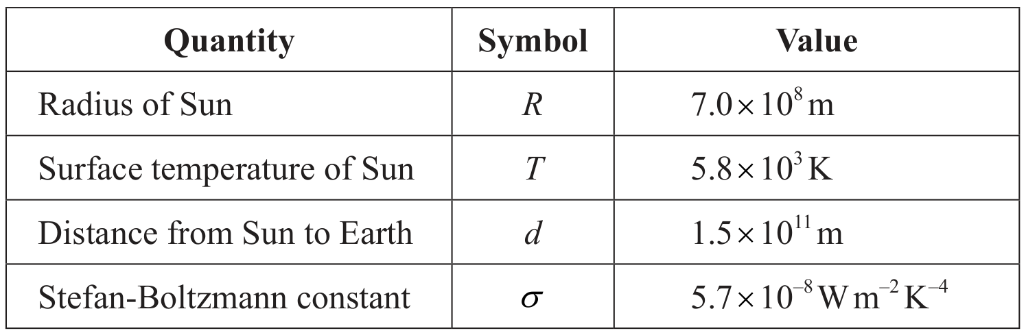
The following data are available.
Outline the conditions necessary for the object to execute simple harmonic motion.
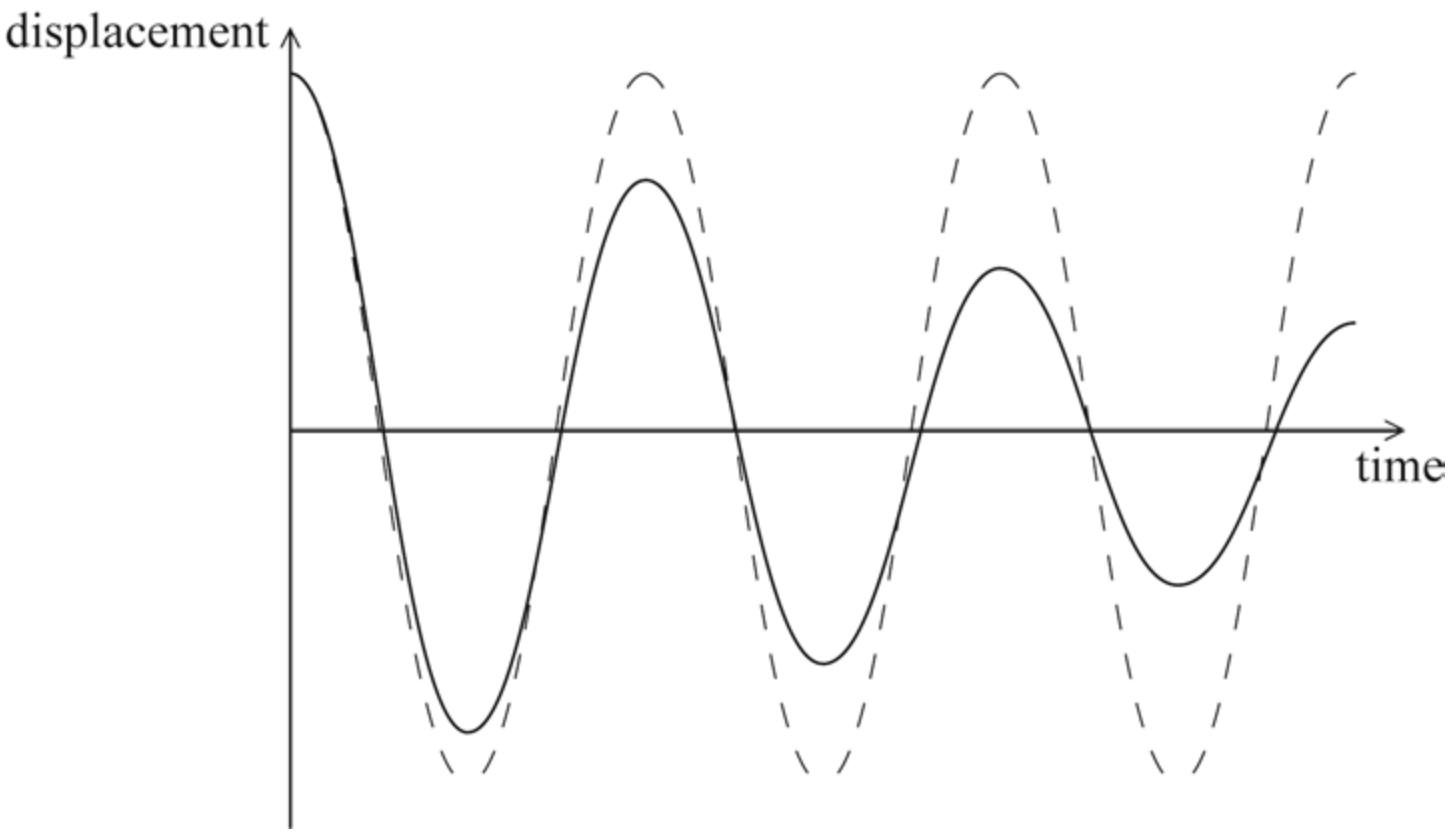
Sketch on the same axes a graph of how the displacement varies with time if a small frictional force acts on the object.
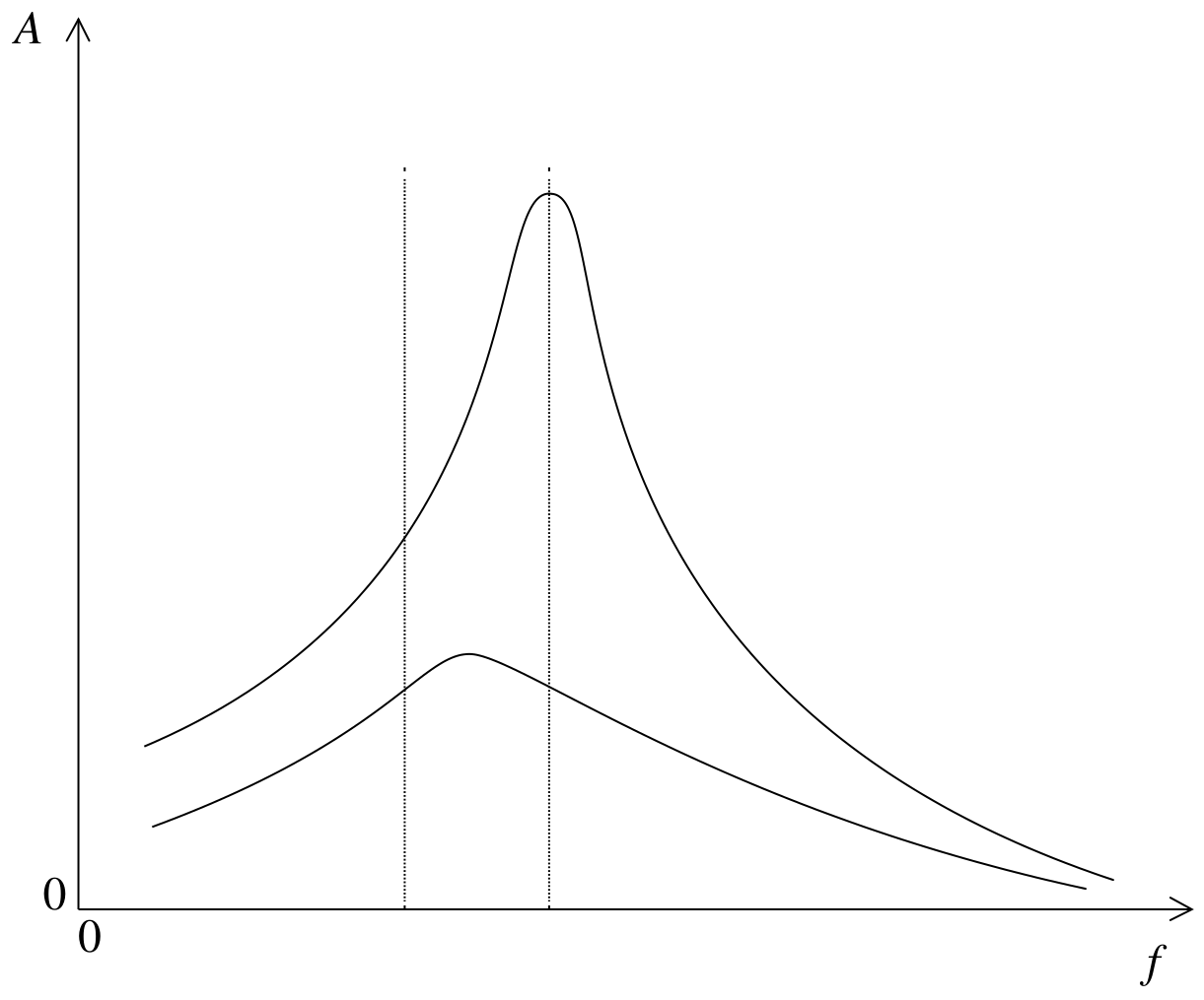
Point P now begins to move from side to side with a small amplitude and at a variable driving frequency f. The frictional force is still small.
At each value of f, the object eventually reaches a constant amplitude A.
The graph shows the variation with f of A.
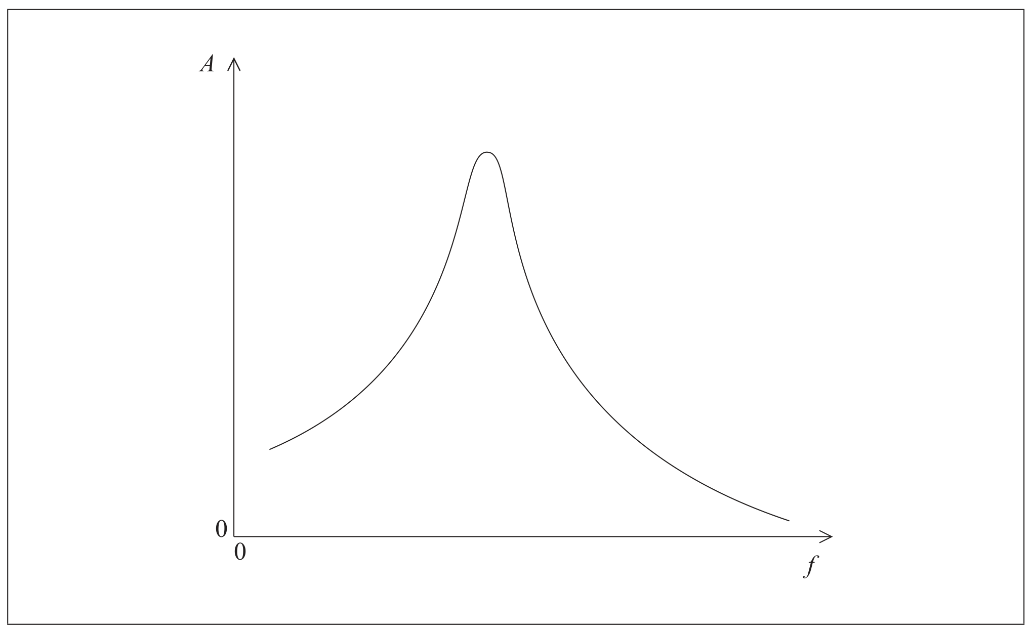
On the same axes, draw a graph to show the variation with f of A when the frictional force acting on the object is increased.