Reactivity 2. How much, how fast and how far?
- Syllabus
- First assessment 2025
- Section
- —
- Level
- HL
A balanced chemical equation conserves every element and charge. Its coefficients show the mole ratio of reactants and products.
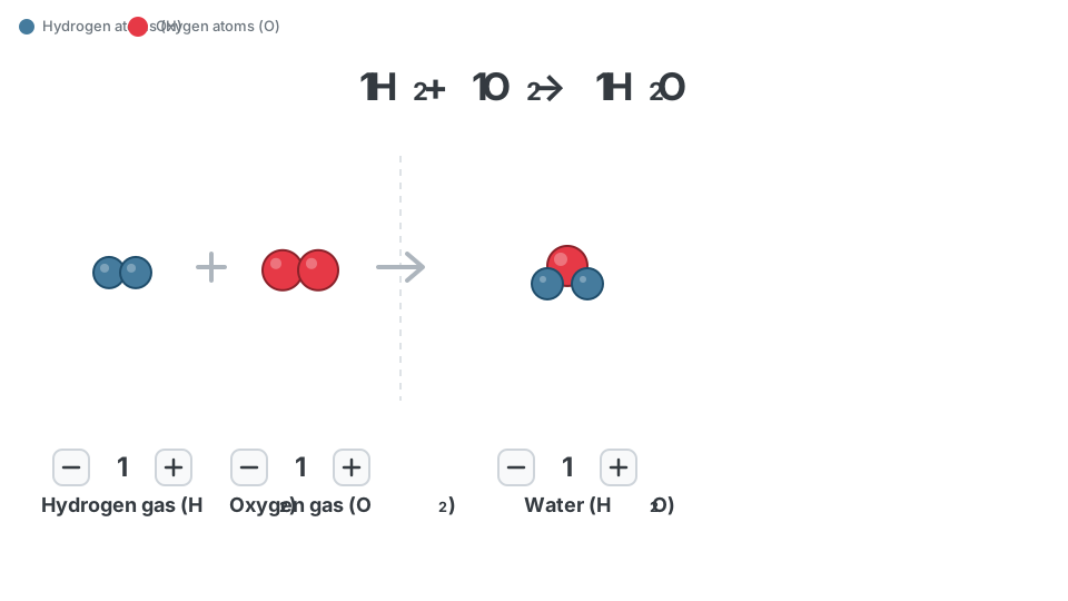
Write the products and state symbols, balance atoms with coefficients rather than changing formula subscripts, then check every element and the charge.
For Al + O₂ → Al₂O₃, preserve the formulas and choose coefficients 4Al + 3O₂ → 2Al₂O₃. Changing O₂ to O or Al₂O₃ to another subscript would change the substances rather than balance them. Add state symbols from chemical evidence or stated conditions, not from atom counting.
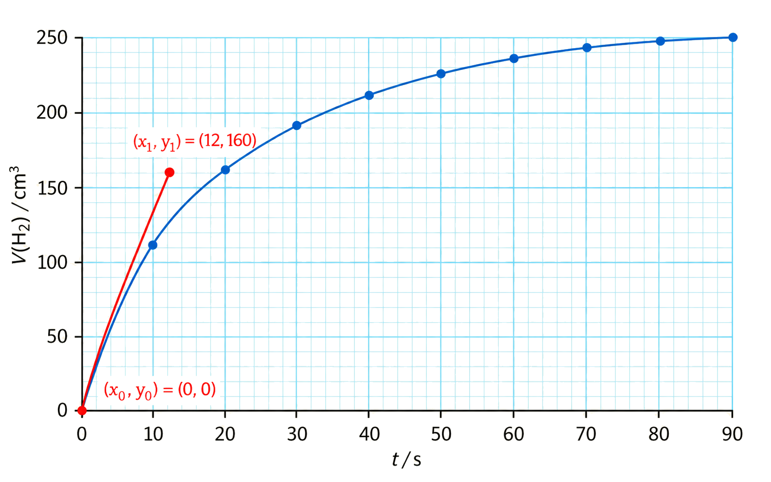
An instantaneous rate is the gradient of a tangent at the stated point on a concentration–time, volume–time or mass–time graph. Keep the units consistent.
Choose two well-separated points on the tangent, not on the curve, to calculate its gradient. A reactant concentration has a negative gradient, so report its disappearance rate as a positive magnitude unless a signed change is requested.
| Requested rate | Graph operation | Evidence check |
|---|---|---|
| mean over an interval | secant gradient between interval endpoints | quote the interval and units |
| initial | tangent gradient at t = 0 | choose well-separated points on the tangent |
| instantaneous at time t | tangent gradient at that time | do not use two points on the curved trace |
A measured mass, pressure or gas volume is a rate proxy only when its change is tied to reaction progress under the stated conditions. Preserve reactant/product slope sign or report a positive disappearance/formation magnitude as requested.
Worked tangent example: on a concentration–time graph for , two points on the tangent at are and . The tangent gradient is . For , divide the positive disappearance-rate magnitude by the HCl coefficient: .
A successful collision needs sufficient kinetic energy to overcome activation energy and a suitable orientation of the reacting particles.
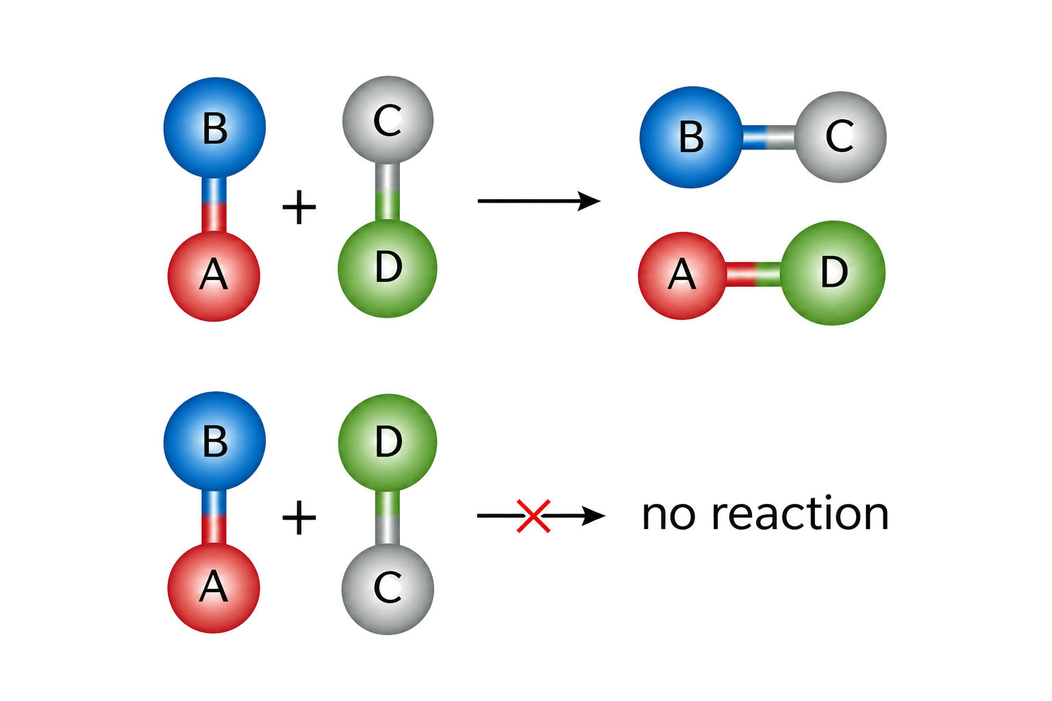
Temperature raises average kinetic energy and changes collision frequency and the fraction of particles with energy at least Ea. Collision frequency alone does not guarantee reaction.
At one temperature, only the fraction of collisions above Ea and with a productive orientation can react. Raising temperature increases that fraction, not the energy of every particle by the same amount. Use collision frequency to explain concentration or pressure effects and the energy distribution to explain the stronger temperature effect.
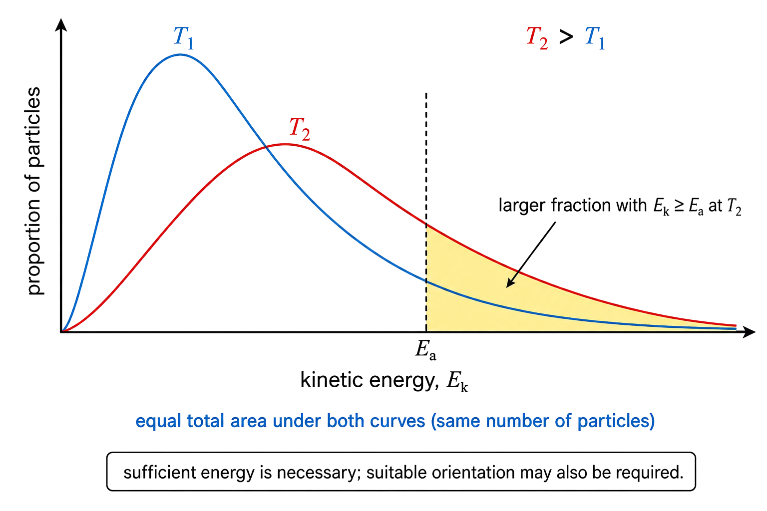
A Maxwell–Boltzmann curve shows the distribution of particle kinetic energies. At higher temperature the peak is lower and shifts right; the area beyond Ea is larger, so more particles can react.
Two Maxwell–Boltzmann curves for the same number of particles have equal total area. At higher T the curve is broader with a lower peak and a larger area to the right of a fixed Ea line; the peak does not move to Ea and no particle count is lost.
A catalyst provides an alternative reaction pathway with lower activation energy. It does not change the energy levels of the reactants or products.
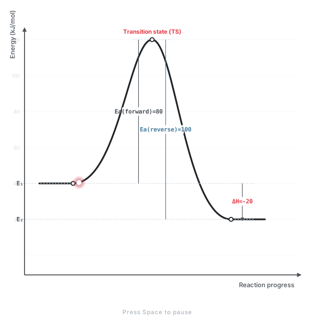
Because the catalysed Ea is lower, a larger fraction of the same distribution lies beyond the threshold. The reaction therefore has more effective collisions at the same temperature.
At fixed temperature a catalyst does not change the Maxwell–Boltzmann distribution; it moves the threshold to a lower Ea, increasing the area beyond it. On an energy profile it changes the pathway and peak, not ΔH, reactant/product energies or the equilibrium constant.
A mechanism is a sequence of elementary steps. The slowest step is the rate-determining step; an intermediate is formed in one step and consumed in a later step, whereas a transition state is the high-energy configuration at a barrier.
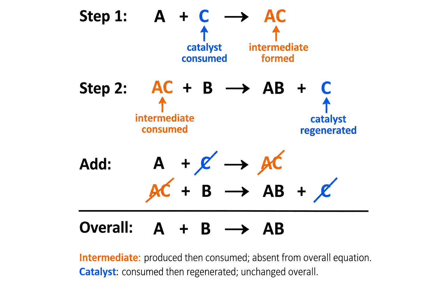
A proposed mechanism must be compared with the experimental rate equation and stoichiometry. Matching a rate equation can support a mechanism but does not prove it, because different mechanisms may give the same expression.
Add all elementary steps and cancel intermediates to recover the overall equation. Then derive the rate dependence expected from the slow step, eliminating an intermediate when necessary, and compare with experiment. A catalyst consumed early and regenerated later cancels from the overall equation but is not an intermediate.
In a multistep profile, peaks are transition states and valleys between peaks are intermediates. Each step has its own Ea; the largest barrier from its preceding intermediate identifies the rate-determining step.
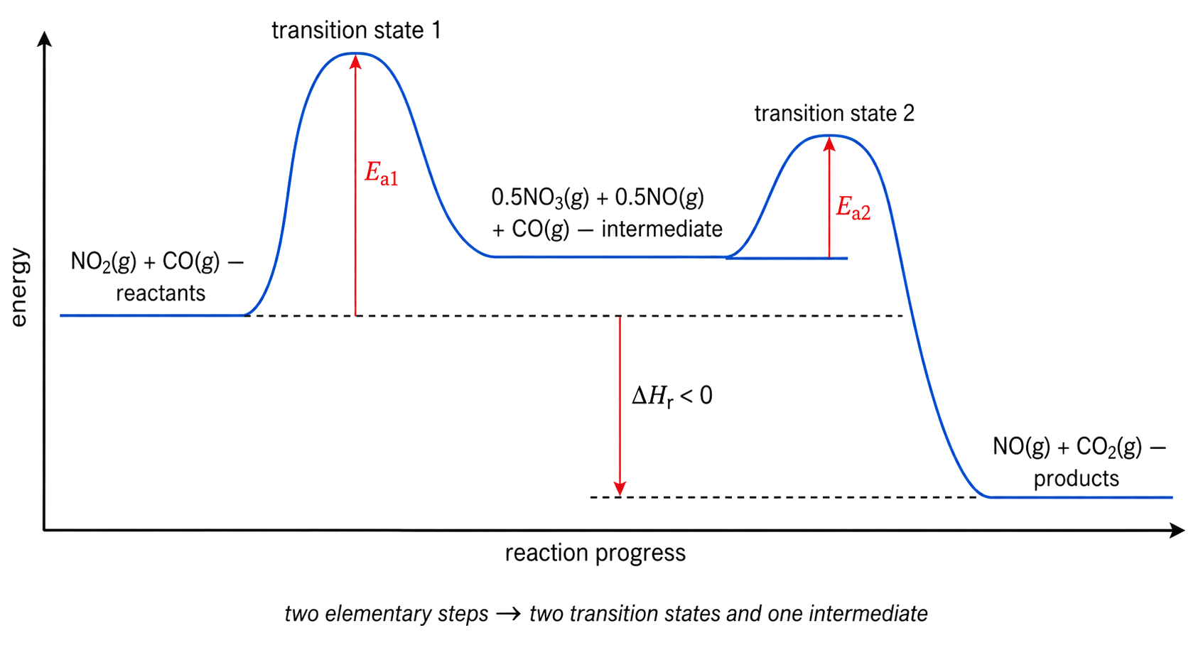
For each step, measure Ea upward from its own preceding reactant or intermediate valley to the next peak. The rate-determining barrier is the largest of those step barriers, which need not be the peak with the greatest absolute height above the page baseline.
![rate-concentration plots are horizontal, linear through origin and parabolic for zero, first and second order; diagnostic linear plots use [A], ln[A] and 1/[A] respectively; slopes are -k, -k and +k respectively; half-life expressions and concentration dependence are correct.](https://cheese-dev-public.oss-accelerate.aliyuncs.com/interactive-content/images/chemistry/ib-knowledge-cards/v1/batch-027/reaction-order-diagnostic-plots-v1.png)
The exponent gives order with respect to that reactant. Use rate factors to identify zero, first or second order, then match the order to the concentration–time or rate–concentration graph.
Use multiple representations as cross-checks: zero-order rate is independent of concentration and [A] falls linearly; first-order rate is proportional to [A] and gives exponential decay; second-order rate curves upward on a rate-versus-concentration plot. Do not infer order from one balanced equation.
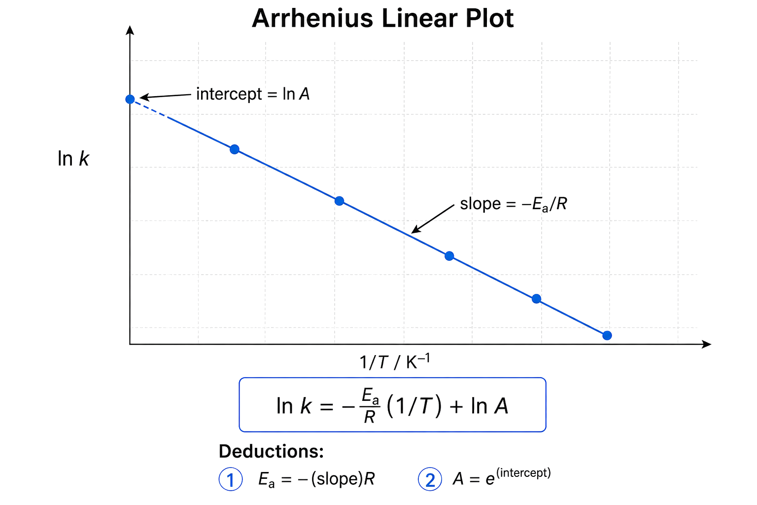
On a plot of ln k against 1/T, gradient = −Ea/R and intercept = ln A. Use kelvin, preserve the negative gradient and convert J mol−1 to kJ mol−1 when required.
A steeper negative ln k versus 1/T gradient means a larger activation energy. When two temperatures are given, subtracting the two linear equations removes ln A and lets Ea be found without knowing the frequency factor.
Worked Arrhenius-plot example: using line points and , the gradient is . Since gradient , . The negative plot gradient therefore produces a positive activation energy.
Dynamic equilibrium occurs in a closed system when the forward and reverse processes continue at equal rates. Macroscopic amounts remain constant, but reactants and products need not be equal in amount.
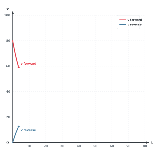
The same rate-balance idea applies to physical equilibria such as vaporization and condensation as well as to reversible chemical reactions.
In a sealed liquid–vapour system at equilibrium, molecules continue evaporating and condensing at equal rates, so pressure and amounts are constant on average. Equal rates do not mean equal concentrations, and opening the system can prevent equilibrium by allowing matter to escape.
An equilibrium shifts to partially counteract an imposed change. Pressure favours the side with fewer gaseous molecules; temperature favours the endothermic direction; concentration changes alter composition.
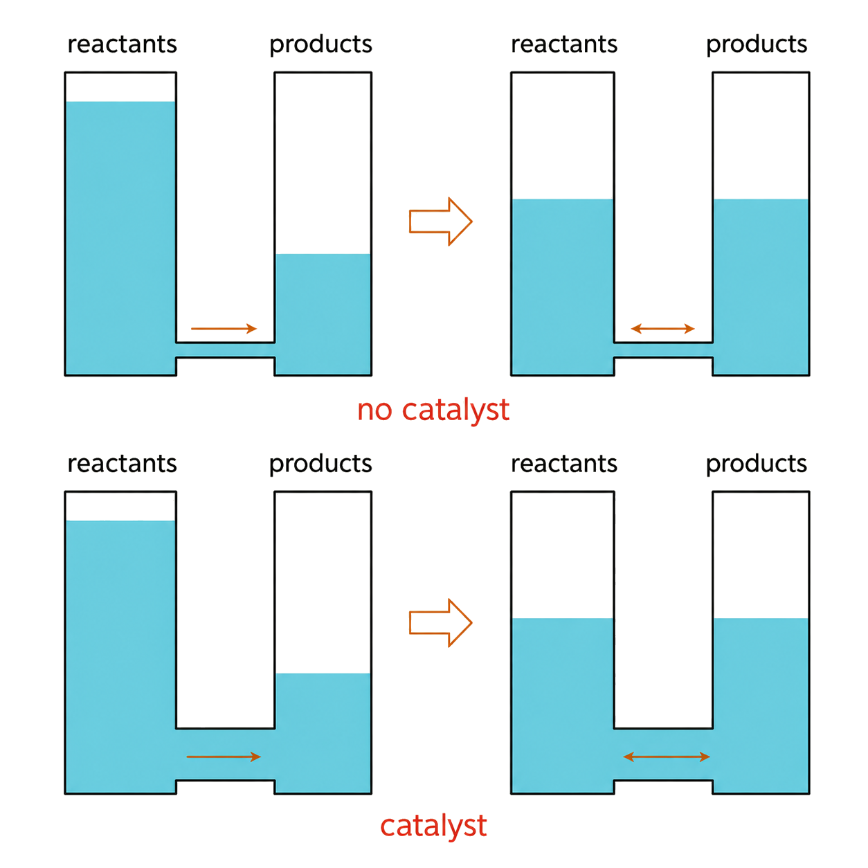
At fixed temperature, concentration and pressure changes do not change K. Temperature changes K. A catalyst changes rates in both directions and does not change equilibrium position.
For N₂(g) + 3H₂(g) ⇌ 2NH₃(g), compression favours the two-mole gas side, but K is unchanged if temperature is fixed. Heating favours the endothermic direction and changes K; a catalyst reaches the same equilibrium faster by accelerating both directions.
| Disturbance | Immediate evidence | K at fixed/new T | Direction check |
|---|---|---|---|
| concentration or pressure change | Q changes before composition readjusts | unchanged if T is fixed | compare the new Q with K |
| raise temperature | heat favours the endothermic direction | K increases if the forward reaction is endothermic; decreases if it is exothermic | use the stated forward ΔH |
| catalyst | both forward and reverse rates increase | unchanged | equilibrium composition is unchanged; it is reached sooner |
For gas pressure, count gaseous coefficients only. Use Q/K or opposing-rate evidence to justify the shift rather than the phrase “counteracts the change” alone.
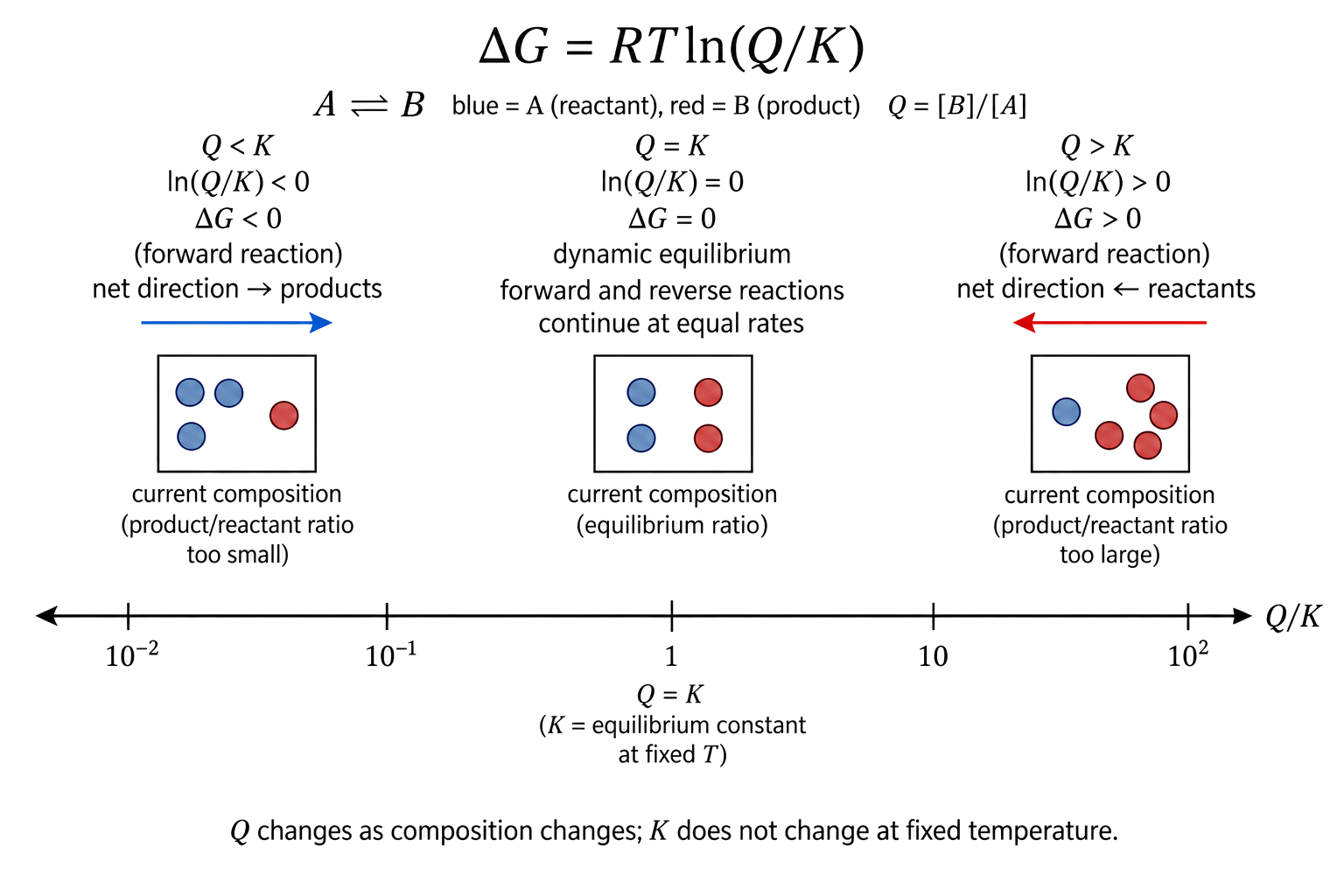
Q uses concentrations at any time, not necessarily equilibrium. Q < K means the forward direction is needed; Q > K means the reverse direction is needed; Q = K means equilibrium.
Calculate Q with the same expression as K but using the current concentrations. If Q = 0.20 and K = 5.0, too little product is present relative to equilibrium, so the forward direction lowers the mismatch. Recalculate after composition changes; Q is a snapshot, not a new constant.
Worked example: for , . If every current concentration is , . At 475 K, , so : the mixture contains too much product relative to equilibrium and the reverse direction is favoured until .
