[Maximum number: 7]

Under controlled driving conditions, Jacob investigated the fuel efficiency of his car when using premium fuel compared to standard fuel.
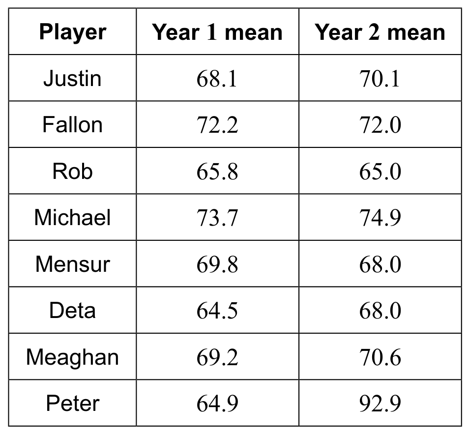
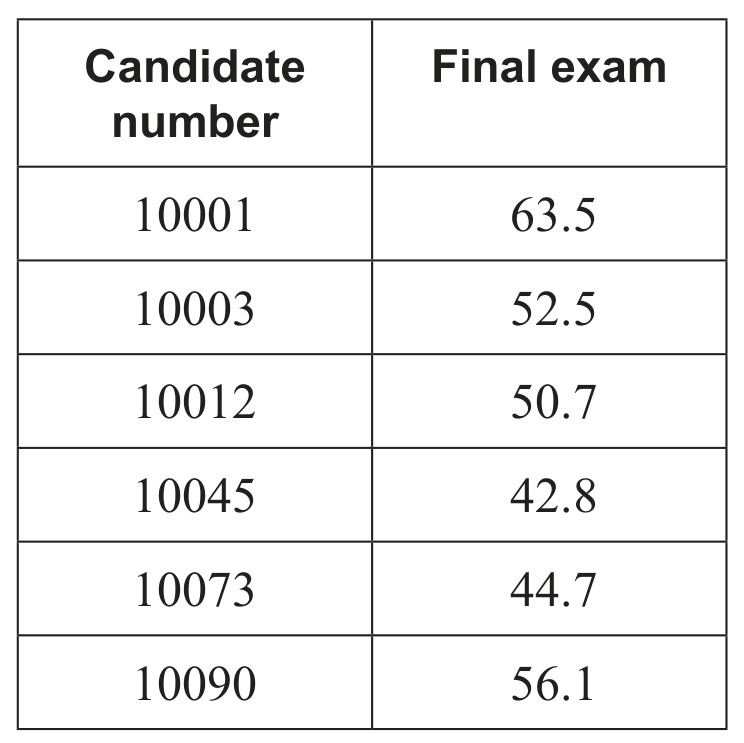
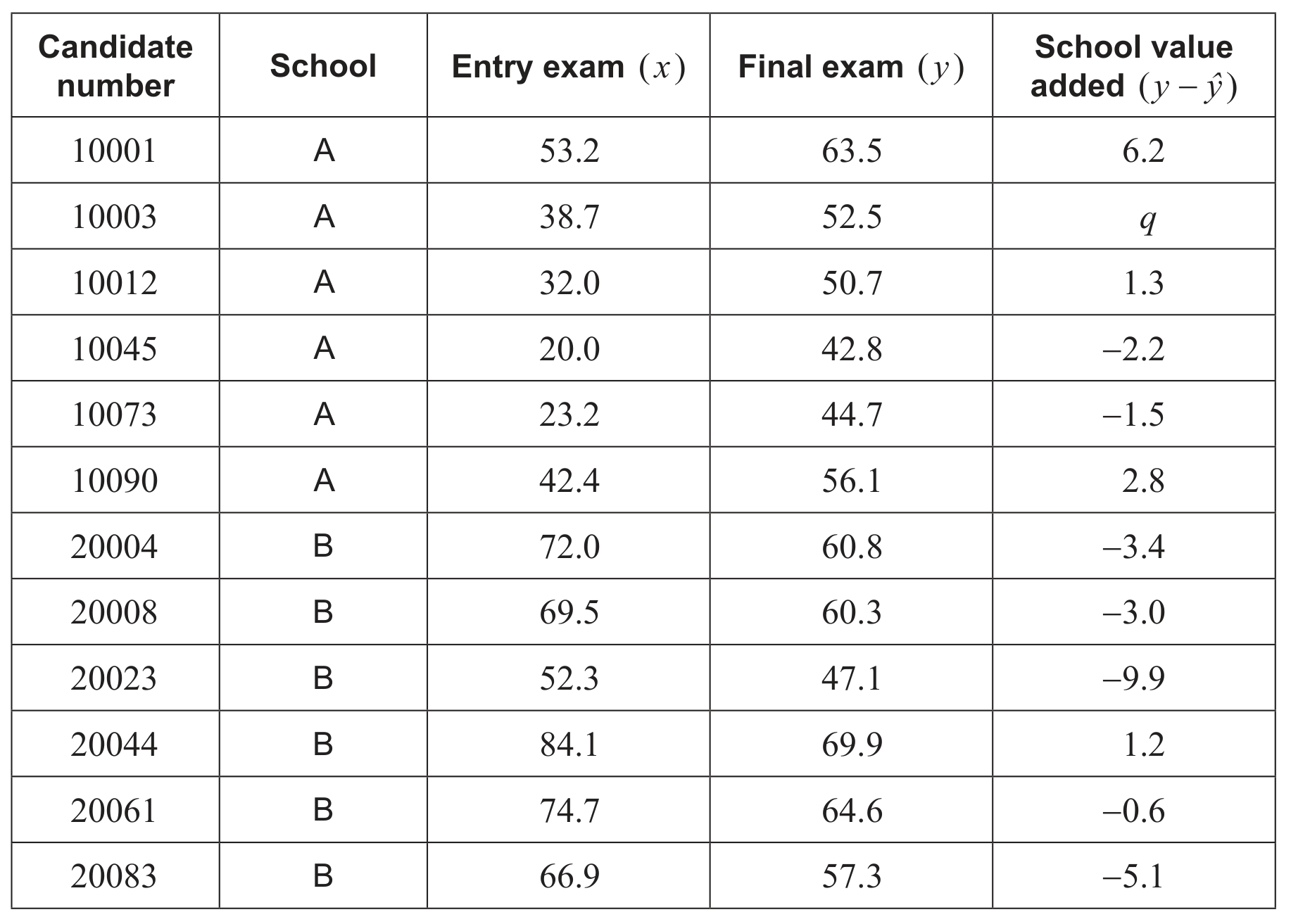
Jacob recorded the distance travelled per litre ( $\mathrm{kmL}^{-1}$ ) using standard fuel for six days and then using premium fuel for seven days. This information is shown in the following tables.

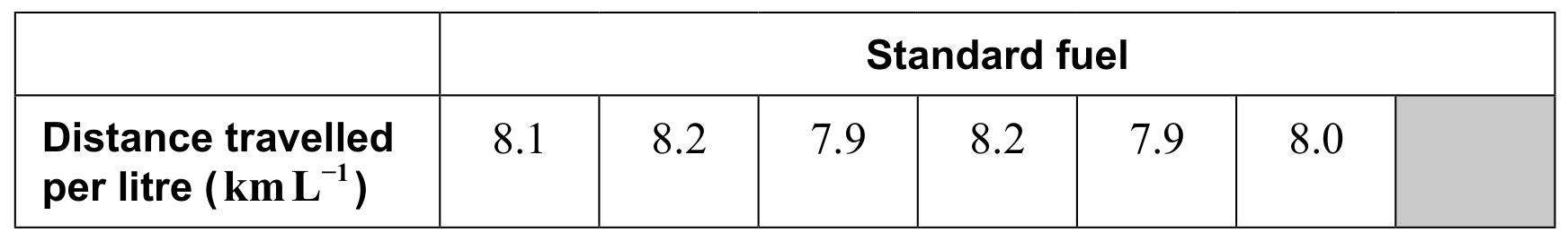
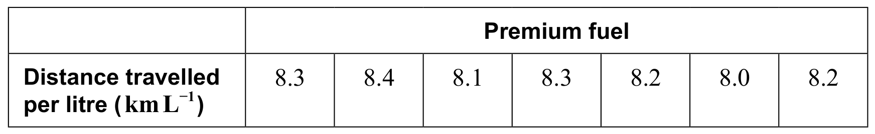
At the 5 % significance level, Jacob performs a t-test to determine whether there is sufficient evidence that his car travels further using premium fuel compared to standard fuel.

(a)

State one mathematical assumption made for this test to be valid.

[ 1 ]

(b)

Write down the

[ 2 ]

(i)

null hypothesis.

(ii)

alternative hypothesis.

[ 2 ]

(c)

(i)

Find the p-value.

(ii)

State your conclusion to the test in context. Justify your answer.

[ 4 ]

[Maximum number: 12]

The following question examines the changes in darts players' scores using two statistical tests.
In the sport of darts, players take turns throwing darts at a board in order to score points.

A player's "three dart average" refers to the mean score achieved when throwing three darts.
Valia aimed to find out whether amateur darts players in her local area improved over a 12-month period. An increase in their "three dart average" would indicate an improvement.

She selected a random sample of eight darts players and recorded their mean "three dart average" from Year 1.

She then recorded their mean "three dart average" from Year 2.
Valia's results were as follows:

Table 1

Valia calculated the median, quartiles and inter-quartile range for each year. The results are shown in Table 2.

Table 2

(a)

Determine the values of a, b and c.

[ 3 ]

(b)

By comparing the results for both years summarized in Table 2, state one conclusion, in context, that Valia might be justified in making.

Valia then decided to analyse the data from Table 1 using a one-tailed paired t-test at the 10 % significance level to determine whether the players' averages have increased.

[ 1 ]

(c)

State an assumption about the differences in means that is necessary in order for the test to be valid.

[ 1 ]

(d)

(i)

State the null and alternative hypotheses for the test.

[ 2 ]

(ii)

Find the p-value.

[ 2 ]

(iii)

State the conclusion of the test in context, justifying your answer.

[ 2 ]

(e)

Suggest briefly how Valia could assess the reliability of her results for either test.

[ 1 ]

[Maximum number: 15]

Dr Petrillo wrote a short scientific essay. He analysed the readability of his essay by counting the number of letters in each word.
Dr Petrillo constructs a box and whisker diagram for his data.

(a)

Write down

[ 3 ]

(i)

the median;

(ii)

the upper quartile, $\mathrm{Q}_{3}$ ;

(iii)

the interquartile range, IQR.

Dr Petrillo now wants to modify his diagram to show any outliers. He considers the longer words in his data and uses the following formula:

\text { outliers }>(1.5 \times \mathrm{IQR})+\mathrm{Q}_{3}

Words with at least k letters are considered outliers.

[ 3 ]

(b)

Find the value of k.

[ 2 ]

(c)

Dr Petrillo further considers the outliers and sees no reason to exclude them from his analysis.
The length of each word in the essay, n, and its associated frequency are given in the following table.

Use the mid-interval values to calculate an estimate of the mean number of letters in each word.

Dr Petrillo conducts a $\chi^{2}$ goodness of fit test at the 1 % significance level, to test the following null hypothesis:
$\mathrm{H}_{0}$ : The frequency of the number of letters in each word in his essay is consistent with the English language.

[ 3 ]

(d)

Write down the alternative hypothesis for this test.

[ 1 ]

(e)

The observed and expected frequencies of the number of letters in each word in his essay are listed in the following table.

[ 4 ]

(i)

Write down the number of degrees of freedom.

(ii)

Find the $\chi^{2}$ statistic for this test.

(iii)

Find the p-value for this test.

The critical value for this test, at the 1 % significance level, is 16.812 .

[ 4 ]

(f)

State whether Dr Petrillo should reject the null hypothesis. Justify your answer.

[ 2 ]

[Maximum number: 14]

A survey was answered by 20000 expatriates (people living in a country that is not their own). The data ranked countries in order of the country they felt was best for expatriates. The highest-ranked country was Switzerland.
These results were compared to happiness scores taken from The World Happiness Report 2022. The following table shows this data for the top 10 expatriate countries.

(a)

For the happiness score, find

[ 4 ]

(i)

the upper quartile

(ii)

the interquartile range.

[ 4 ]

(b)

Show that Switzerland's happiness score is not an outlier for this data.

[ 3 ]

(c)

The happiness scores were ranked to calculate Spearman's rank correlation coefficient, $r_{s}$ . These ranks are shown in the following table.

Write down the value of

[ 3 ]

(i)

a

(ii)

b

(iii)

c.

[ 3 ]

(d)

(i)

Find $r_{s}$ .

(ii)

If France's happiness score is upgraded to 6.9 , explain why the value of $r_{s}$ does not change.

Jose concludes from this data that countries with high happiness scores are likely to be favourite expatriate countries.

[ 3 ]

(e)

State, with a reason, whether Jose's conclusion is appropriate.

[ 1 ]

[Maximum number: 3]

In this question you will use graph theory and transition matrices to solve problems about a manager visiting five factories.
Audrey is the quality control manager for a manufacturing company that has five factories, A, B, C, D and E .
She is planning a route to visit each factory once, starting and finishing from her home, H .
She determines the distance between each location, in kilometres, as shown in the table.

Audrey wants to find an upper and lower bound for the shortest total distance travelled on her route.

(a)

Over a long period of time,

[ 3 ]

(i)

find the expected distance Audrey travels in a day, given that she always travels directly from home to a factory and then back home.

[ 3 ]

[Maximum number: 18]

Juliet is a sociologist who wants to investigate if income affects happiness amongst doctors. This question asks you to review Juliet's methods and conclusions.
Juliet obtained a list of email addresses of doctors who work in her city. She contacted them and asked them to fill in an anonymous questionnaire. Participants were asked to state their annual income and to respond to a set of questions. The responses were used to determine a happiness score out of 100 . Of the 415 doctors on the list, 11 replied.

(a)

(i)

Describe one way in which Juliet could improve the reliability of her investigation.

[ 1 ]

(b)

Juliet classifies response K as an outlier and removes it from the data. Suggest one possible justification for her decision to remove it.

[ 1 ]

(c)

For the remaining ten responses in the table, Juliet calculates the mean happiness score to be 52.5.

[ 4 ]

(i)

Calculate the mean annual income for these remaining responses.

[ 2 ]

(ii)

Determine the value of r, Pearson's product-moment correlation coefficient, for these remaining responses.

Juliet decides to carry out a hypothesis test on the correlation coefficient to investigate whether increased annual income is associated with greater happiness.

[ 2 ]

(d)

(i)

State why the hypothesis test should be one-tailed.

[ 1 ]

(ii)

State the null and alternative hypotheses for this test.

The critical value for this test, at the 5 % significance level, is 0.549 . Juliet assumes that the population is bivariate normal.

[ 2 ]

(iii)

Determine whether there is significant evidence of a positive correlation between annual income and happiness. Justify your answer.

[ 2 ]

(e)

Juliet wants to create a model to predict how changing annual income might affect happiness scores. To do this, she assumes that annual income in dollars, X, is the independent variable and the happiness score, Y, is the dependent variable.

She first considers a linear model of the form

Y=a X+b

[ 2 ]

(i)

Use Juliet's data to find the value of a and of b.

[ 1 ]

(ii)

Interpret, referring to income and happiness, what the value of a represents.

Juliet then considers a quadratic model of the form

Y=c X^{2}+d X+e

[ 1 ]

(f)

(i)

State the name of the test which Juliet should use.

[ 1 ]

(ii)

State the null and alternative hypotheses for this test.

[ 1 ]

(iii)

Perform the test, using a 5 % significance level, and state your conclusion in context.

[ 3 ]

[Maximum number: 18]

Paul has a bar graph for the total number of goals scored in each game of a soccer tournament in 2024. The bar graph is shown below, however the frequency of 4 goals in a game is unreadable.
Paul uses this bar graph to create a frequency table.

Frequency table

(a)

Write down the value of k.

Paul knows that the mean number of goals per game scored during the tournament was 2.2 .

[ 1 ]

(b)

(i)

Write down an equation for the mean in terms of p.

[ 3 ]

(ii)

Determine the value of p.

Data for the number of goals per game in the 2025 soccer tournament are shown in the following box and whisker diagram.

After comparing the box and whisker diagram from the 2025 tournament with the frequency table from the 2024 tournament, Paul concludes that the distribution of goals is consistent between the two tournaments.

[ 3 ]

(c)

State two observations that support Paul's conclusion using values from the data to compare any two of:
range, symmetry, median, and interquartile range.

Paul plans to watch all the games from the 2024 tournament in a random order.
He will watch each game once.
For the first game he watches, he defines event F as:
"scoring either 0 goals or exactly 1 goal".

[ 3 ]

(d)

Write down the event(s) from the table that are equivalent to $F^{\prime}$ . There may be more than one correct event.

[ 2 ]

(e)

If exactly 1 goal was scored in the first game Paul watches, write down the probability that exactly 1 goal was scored in the second game he watches. Give your answer as a fraction.

[ 2 ]

(f)

Calculate the probability that 5 goals were scored in the first game that Paul watches and 0 goals were scored in the second game he watches.

[ 4 ]

[Maximum number: 25]

This question is about comparing the academic performance of two schools.
At age 18, all students in school A and school B take the same final exam. Augustin is studying the results in these schools.
Augustin chooses to take a representative sample of size six from each school. For each student in the sample, he will conduct an interview.

(a)

(i)

State one advantage of increasing the sample size.

[ 1 ]

(ii)

State one disadvantage of increasing the sample size.

The data in Table 1 shows the results of the final exam as a percentage for each of the six students, sampled from school A.

Table 1

The mean result for the sample from school A is 51.7 to three significant figures.

[ 1 ]

(b)

Find the value of $s_{n-1}$ for the sample from school A.

The value of $s_{n-1}$ for the sample from school B is 7.66 to three significant figures.
Augustin makes the following claim:
"The spread of results in school A must be less than the spread of results in school B."

[ 2 ]

(c)

Make one criticism of Augustin's claim.

The examination board claims that the final exam results in each school are approximately normally distributed. You may assume that this claim is correct.

Augustin decides to use a pooled t-test to compare the mean results of school A and of school B.

[ 1 ]

(d)

(i)

State the condition regarding population variances required to use a pooled t-test.

[ 1 ]

(ii)

State whether Augustin should use a pooled t-test in this case. Justify your answer.

Prior to collecting data, Augustin believed that the mean result of school B was higher than that of school A. From his data he finds that the mean final exam result for the sample from school B is exactly 60.

[ 2 ]

(e)

(i)

State appropriate null and alternative hypotheses for the pooled t-test.

[ 2 ]

(ii)

Find the p-value.

[ 2 ]

(iii)

Given that the test is carried out at the 5 % significance level, state the appropriate conclusion in context. Justify your answer.

All students in the two schools took the same entry exam at age 11.
Augustin wants to determine if there is evidence of any correlation between the entry exam result and final exam result. For the 12 students in the sample, Augustin collects their entry exam results.

The Pearson's product moment correlation coefficient between the results for the entry exam and the final exam is r=0.876 to three significant figures. The critical value of r at the 5 % significance level is 0.576 .

[ 2 ]

(f)

(i)

Assuming all requirements are met, perform a test at the 5 % significance level. State the hypotheses and justify your conclusion.

[ 4 ]

(ii)

If the requirements are not met, state an alternative test.

The examination board uses a model to make a prediction of a student's final exam result ( $\hat{y}$ ) based on their entry exam result ( x ).

The model used is:

\hat{y}=0.37 x+37.6

[ 1 ]

(g)

For each student, Augustin uses the value $y-\hat{y}$ rounded to one decimal place to measure the extent to which a school helped to improve a student's results. He calls this "school value added". This is shown in Table 2.

Table 2

[ 4 ]

(i)

Assuming that the appropriate requirements are met, use a pooled t-test at a 5 % significance level to determine if the mean "school value added" is higher in school A than in school B. Write down your null and alternative hypotheses and justify your conclusion.

[ 4 ]

(h)

Using Augustin's results, explain how each school could claim they are performing better than the other school.

[ 2 ]

[Maximum number: 10]

This question considers how the assessment of the Air Quality Index (AQI) for a school depends on the method chosen by the person doing the assessing.
Air quality for a district is measured at three monitoring stations. The positions of these stations on a coordinate system with units in kilometres are A(0,5), B(8,9) and C(8,1).
A Voronoi diagram is constructed with the three stations as sites.

(a)

Explain why the principal might not accept that the air quality around the school can be classed as "good".

The principal decides to obtain an expected value for the AQI at the school that uses all the available information. To do this, she uses an alternative method: the natural neighbour algorithm. This algorithm has two stages.

The first stage is to create a new Voronoi diagram with the school as an extra site. This is shown in the following diagram with the edges of the previous diagram shown by dashed lines.

The second stage is to estimate the AQI value at the school, W, by using the formula

W=\frac{w_{A} a_{A}+w_{B} a_{B}+w_{C} a_{C}}{T}

In the formula, $a_{A}$ is the area within the new cell that has been taken from the cell surrounding site A , shown as region P on the diagram, and $w_{A}$ is the mean AQI value from site A . This is given as 132 in the table of mean AQI values above. Similarly for sites B and C . T is the total area of the new cell around S .

[ 1 ]

(b)

Test at the 10 % significance level the hypothesis that the mean AQI value at the school is greater than 94.4. State clearly the null and alternative hypotheses and the conclusion of the test in context.

The principal now assumes that the distribution of AQI values at the school follows a normal distribution with mean 97.8 and standard deviation 17.2.

[ 6 ]

(c)

Use this model to find the expected number of days per year (correct to the nearest day) on which the AQI value can be classed as "good".

[ 3 ]

[Maximum number: 4]

This question considers whether it is reasonable to go on all the rides in a theme park and get back to the entrance in two and a half hours.
Martin is visiting a theme park. He will enter the park at 09:00 and must leave the park by 11:30. He uses information available on the internet to calculate whether he will be able to go on all of the rides in the two and a half hours.
He begins by constructing a graph which shows the main paths between the rides and the route of the cable car between the entrance/exit A and ride D.
His graph and the names of the rides are shown in the following diagram.

The weights on the edges of the graph represent the times, in minutes, to walk between the rides and the time to travel by cable car between A and D.

Let T be the shortest possible time, in minutes, taken to visit all the rides, beginning and ending at A .

Martin notices that the graph contains a Hamiltonian cycle. He decides to use the weight of the Hamiltonian cycle as an upper bound for T.

(a)

(i)

Find the probability that Martin manages to go on all five rides and return to the entrance in two and a half hours.

Martin enters the park at 09:00 and decides to follow his planned route, but has two consecutive rides on Energy Pulse.

[ 4 ]

Question 1

Question 1(a)

Question 1(b)

Question 1(b)(i)

Question 1(b)(ii)

Question 1(c)

Question 1(c)(i)

Question 1(c)(ii)

Question 1

Question 1(a)

Question 1(b)

Question 1(c)

Question 1(d)

Question 1(d)(i)

Question 1(d)(ii)

Question 1(d)(iii)

Question 1(h)

Question 1

Question 1(a)

Question 1(a)(i)

Question 1(a)(ii)

Question 1(a)(iii)

Question 1(b)

Question 1(c)

Question 1(d)

Question 1(e)

Question 1(e)(i)

Question 1(e)(ii)

Question 1(e)(iii)

Question 1(f)

Question 1

Question 1(a)

Question 1(a)(i)

Question 1(a)(ii)

Question 1(b)

Question 1(c)

Question 1(c)(i)

Question 1(c)(ii)

Question 1(c)(iii)

Question 1(d)

Question 1(d)(i)

Question 1(d)(ii)

Question 1(e)

Question 1

Question 1(e)

Question 1(e)(ii)

Question 1

Question 1(a)

Question 1(a)(i)

Question 1(b)

Question 1(c)

Question 1(c)(i)

Question 1(c)(ii)

Question 1(d)

Question 1(d)(i)

Question 1(d)(ii)

Question 1(d)(iii)

Question 1(e)

Question 1(e)(i)

Question 1(e)(ii)

Question 1(f)

Question 1(f)(i)

Question 1(f)(ii)

Question 1(f)(iii)

Question 1

Question 1(a)

Question 1(b)

Question 1(b)(i)

Question 1(b)(ii)

Question 1(c)

Question 1(d)

Question 1(e)

Question 1(f)

Question 1

Question 1(a)

Question 1(a)(i)

Question 1(a)(ii)

Question 1(b)

Question 1(c)

Question 1(d)